A review of "Refining deep generative models via discriminator gradient flow" by Vira Koshkina and Myles Doyle.

TL;DR: The paper proposes an iterative scheme for refining latent samples in GANs. The refinement is done by iteratively computing the gradient of the f-divergence loss evaluated at a sample generated by the generator and discriminated by the discriminator with an added noise term that introduces stochasticity. These updates move the latent in the direction that minimises the loss, meaning it improves the quality of the images generated from the latent by ensuring that it looks more realistic to the discriminator.  

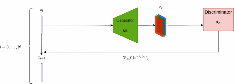
Schematic overview of the iterative latent refinement scheme using discriminator gradient flow. 

Introduction

Deep generative models (DGMs) excel at generating realistic images that closely resemble real-world images. Generative Adversarial Networks (GANs) [1] are now a commonly used type of DGM that boasts the ability to produce high-quality images resembling real data. GANs are a likelihood-free method that consists of a generator and discriminator. The generator is trained to produce data similar to real data (in our case, images), while the discriminator is trained to distinguish real data from ones that the generator created. After training is complete, the generator can be used to simulate data while the discriminator is typically discarded.

However, discarding the discriminator has been shown to be wasteful as it contains information about the underlying distribution of the data the model was trained with. This has led to various sample improvement techniques that use the information contained in the discriminator to help improve the quality of the generator's samples [2-5]. These techniques have several drawbacks as they either;

• have wasteful rejection operations in the data space
  
  
• use a sensitive diffusion term to ensure sample diversity
  
  
• only improve GANs with scalar-valued discriminators, excluding those with vector-valued critics and likelihood-based generative models

In this paper, Discriminator Gradient flow (DG flow) is introduced as a method that completely removes the above restrictions. DG flow is used to refine samples by using the gradient flow in the Wasserstein space of f-divergences between the generated image distribution and the real image distribution.

The paper also generalizes DG flow to a variety of DGMs given a pre-trained discriminator. It can be applied to various types of DGMs including; GANs with vector-valued critics, likelihood-based models such as Variational Autoencoders (VAEs), and Normalizing Flows.

Before we dive into how DG flow works, we first need to cover some background theory. We begin in the Euclidean space by defining a gradient flow and how the Euler solver can approximate a solution to a gradient flow given an initial condition. We then define an iterative solver for a stochastic process. Finally, the gradient flow of f-divergences in the Wasserstein space will be described. The gradient flow of f-divergence in the Wasserstein space provides the backbone of the DG flow method that is introduced in the paper.

Gradient Flows

Let $$(X, | |\cdot| |)$$ be a Euclidean space and $$F: X -> \textbf{R}$$ be a smooth function. The gradient flow (or steepest descent curve) of $$F$$ is the smooth curve $$\{x_t\}_{t\;\varepsilon\; \mathbb{R}\;_+}$$ such that

$$ \begin{cases} \mathbf{x}'(t) = -∇ F(\mathbf {x}(t) \\ \mathbf {x}(0) =\mathbf {x}_0 \end{cases}$$

where  $$∇$$ denotes gradient.  Thus, the gradient flow defines a smooth curve that follows the direction of the steepest descent. $$F$$ is minimized along this curve of steepest descent.

Euler Method for Gradient Flows

In general, an ODE

$$\frac{dx(t)}{dt} =a(x(t),t)$$

with an initial value $$a(x(0),0) = a_0$$, can be solved numerically over a continuous time interval $$[0,T]$$ by iterating over the Euler method for $$N$$ steps;

$$x_{i+1} = x_i + h a(x(t),t)$$

where the stepsize $$h = Δ t = \frac{T}{N}> 0$$.

The gradient flow of $$F$$ defined above is an ODE. Thus, we can apply the forward Euler method to obtain an approximate solution with $$a(x(t),t) = -∇ F(\mathbf {x}(t))$$. Therefore, the Euler update step for gradient flows is defined as

$$x_{i+1} = x_i - \;h\; ∇\; F\;(\mathbf {x}_t)$$,

and the system can be solved for small step sizes as $$h \rightarrow 0$$.

Euler-Maruyama  Method

As we will see later, we will need to solve a system that has an extra term added to our gradient flow. This extra term is a type of stochastic process called a Wiener process. Unfortunately, this makes solving the system more complicated, as we will now need to solve a Stochastic Differential Equation (SDE). To do this, we use the Euler-Maruyama method (also called the Euler method). In this section, we will introduce the Euler-Maruyama method and then apply it later.

But first, we define a standard one-dimensional Wiener process $$W_ t\;\varepsilon\; \mathbb{R}$$ (also known as Brownian motion) as a real valued continuous-time stochastic process such that

• $$W_0 = 0$$
  
  
• $$W_t - W_s$$ is independent of $$\{W_\tau\}\;_{\tau \;≤ \;s} \;∀0≤s< t$$ (ie. non overlapping increments are independent)
  
  
• The distribution of $$W_t - W_{t-s}$$ is independent of $$s$$
  
  
•  An increment $$W_t - W_s$$ is a Gaussian process with mean $$0$$ and variance $$t-s$$ $$∀0≤s \lt t$$
• The function mapping $$t$$ to $$W_t$$ is continuous in $$t$$ with probability $$1$$

Furthermore, a $$d$$-dimensional Wiener process $$\mathbf {W}_t = (W_t^{(1)}, W_t^{(2)},\ldots, W_t^{(d)})$$ is a vector valued stochastic process whose components $$W_t^{(i)}$$ are one-dimensional Wiener processes and are independent of each other for $$i=1,2,\ldots, d$$.

Now, consider the stochastic differential equation (SDE)

$$dX_t = a( X_t, t) dt + b( X_t,t) d W_t$$

with the initial condition $$X_0 = x_0$$ and where $$d \mathbf {W}_t$$ is a Wiener process. To solve this SDE on a time interval $$[0, T]$$, we can apply the Euler-Maruyama method to iteratively approximate the true solution $$X$$. To do this we

• split our time interval $$[0,T]$$ into $$N$$ equal non-overlapping subintervals $$\tau_1, \tau_2 , \ldots, \tau_n$$of width $$\Delta t = \frac{T}{N} \gt 0$$ such that

                $$0 = \tau_1 \lt \tau_2 \lt \ldots \lt \tau_n = T$$

• set $$Y_0 = X_0$$
  
  
• Recursively apply the following iterative solver for $$i = 0, \ldots, N-1$$ and for $$\Delta W_i = W_i - W_{i-1}$$: 

                $$Y_{i+1} = Y_i + a(Y_{i}, \tau_i) \Delta t + b(Y_{i}, \tau_i) \Delta W_i$$

As $$N$$ becomes large $$t \rightarrow 0$$ and $$X_N = Y_N \rightarrow X$$. Our solver approximates the stochastic process and therefore approximates a solution $$X_N \approx X$$.

How gradient flows work in Wasserstein Space 

Moving from the Euclidean Space to Wasserstein Space we first have to define our functional $$F$$ operating in the space of probability measures  $$F(\rho): P_2(\Omega) \rightarrow \mathbb {R}$$.  

For this functional we can write a PDE analogues the one above that describes the gradient flow as:

$$v_t (x) = −∇ _x \left(\frac {\delta F}{\delta \rho} \right)$$ ,

where $$v_t$$ is the velocity field at $$\rho_t$$ and $$\frac{\delta F}{\delta \rho}$$ is the first variation of the functional F. 

The curve $$\{\rho_t\}$$ then describes the gradient flow.  We can then write out the continuity equation for the flow $$\{\rho_t\}$$: 

$$∂_t \rho_t + ∇\cdot (\rho_t v_t ) = 0$$

$$∂_t \rho_t- ∇\cdot \left(\rho_t  ∇ \left( \frac{\delta F}{\delta \rho} \right)\right) = 0$$

This continuity equation is the PDE that describes the gradient flow of the functional $$F$$ in the $$W_2$$ space.  The precise derivation of this statement can be found in [9], section 4.3. 

Generator refinement via Discriminator Gradient Flow

Now that we have all the background information we need, we can construct the entropy-regularised f-divergence functional $$F_\mu^{f}(\rho): P_2(\Omega) \rightarrow \mathbb{R}$$ as

$$F_\mu^{f}(\rho)\; {\triangleq }\;  D_{f} (\mu |\ | \rho) - \gamma \;  H (\rho) {\triangleq}\underbrace{\int f\left(\frac{\rho(\mathbf {x})}{\mu(\mathbf {x})}\right)\mu(\mathbf{x}) d \mathbf {x})}_\text{f-divergence} + \underbrace{\; \gamma  \int \rho(\mathbf {x}) \log \rho(\mathbf {x}) d  \mathbf {x})}_\text{negative-entropy}$$,

where $$f$$ is a twice differentiable convex function with $$f(1) = 0$$, and $$\gamma$$ is a scalar coefficient that sets how strong the entropy term is [8]. Note, the symbol $$\triangleq$$ in the above equation means 'equal by definition'. The f-divergence term ensures the distance between the generated image distribution $$\rho$$ and true image distribution $$\mu$$ decrease along the gradient flow.

The entropy term is included above as, by itself, the f-divergence term (Wasserstein distance) does not converge well to the optimal solution, especially when compared to the Optimal Transport optimisation method [9]. Without the entropy term, the f-divergence has the effect of matching one point in the generated image distribution $$\rho$$ to one point in the true image distribution $$\mu$$. Regularising our f-divergence functional with an entropy term with coefficient $$\gamma$$, $$F$$ will then map a point in our generated image distribution $$\rho$$ to a region in our true image distribution $$\mu$$. The region in the true image distribution increases with $$\gamma$$. This has been shown to drastically increase sample accuracy for simulating gradient flow in finite steps [9]. For more details on this, I recommend having a look at this video.

The gradient flow of $$F_\mu^{f}(\rho)$$ in the Wasserstein space $$(P_2(\Omega), W_2)$$ is the following PDE [10],

$$∂_t \rho_t(\mathbf {x}) - ∇_{\mathbf {x}}\cdot \left(\rho_t(\mathbf {x})∇_{\mathbf {x}} f'\left(\frac{\rho_t(\mathbf {x})}{\mu (\mathbf {x})}\right)\right) - \gamma \Delta_{\mathbf {xx}} \rho_t(\mathbf {x}) = 0$$,

where $$∇\cdot$$ and $$\Delta_{\mathbf{xx}}$$ are the divergence and Laplace operators respectively.

The PDE above is of a specific form (Focker-Planck equation to be specific) which has a SDE counterpart [11], given by

$$d \mathbf x_{t} = -\; ∇\;_\mathbf {x}f'\left(\frac{\rho_t}{\mu}\right) (\mathbf {x}_t) dt  + \sqrt{2 \gamma} d\mathbf{w}_t,$$

where $$d \mathbf {w}_t$$ is the standard Wiener process.

This equation defines the evolution of a point (or in our case, an image) $$\mathbf {x}_t$$ as a type of non-linear stochastic process, as the first term depends on the distribution $$\rho_t$$ of point $$\mathbf {x}_t$$ at any time $$t$$. The distribution of $$\mathbf {x}_t$$ in  the above SDE solves the previous PDE. This SDE is of the same form as the SDE described in the above section on the Euler-Maruyama Method with 

$$a(X(t),t) =-∇_{\mathbf {x}}f'\left(\frac{\rho_t}{\mu}\right) (\mathbf {x}_t)   $$,

and

$$b(X(t),t) = \sqrt{2 \gamma}.$$

Thus, we can write our Euler update step as

$$\mathbf {x}_{\tau_{n+1}} = \mathbf {x}_{\tau_{n}} - \eta ∇_{\mathbf {x}} f'\left(\frac{\rho_{\tau_n}}{\mu}\right)(\mathbf {x}_{\tau_n}) + \sqrt{2 \gamma \eta } \mathbf {ξ}_{\tau_n},$$

where $$\mathbf ξ_{\tau_n} \thicksim \eta (\mathbf {0},\mathbf {I})$$, the time interval $$[0,T]$$ is partitioned into equal intervals of size $$\eta$$ and strictly monotomic discretised timesteps $$\tau_i$$ (ie. $$\tau_0 < \tau_1 < \ldots < \tau_N$$).

In fact, we can sample from $$\rho_t$$ by first choosing an initial condition $$\mathbf {x}_0 = \rho_0$$ and then iteratively improve our sample $$x_i$$ by approximately simulating the SDE for each update step.

The above equation now gives us a non-parametric way to improve our generated image samples. Specifically, relating this back to our GANs implementation; let $$g_{\theta}$$ be our generator obtained by sampling from $$\mathbf {z} \thicksim p_Z(\mathbf {z})$$ (sampling from our prior latent distribution) and then passing this sample $$\mathbf {z}$$ into $$g_{\theta}$$. This gives us an initial approximation $$\mathbf {x}_0 \sim \rho_{\tau_0}$$ from our generator $$g_{\theta}$$. The update step outlined in the above equation can then be iterated $$N$$ times to refine our initial approximation.

Assuming we have a binary discriminator $$D$$ that has been pre-trained to distinguish samples $$\mathbf {x} $$ from our true image distribution $$\mu$$ and our generated samples from distribution $$\rho_{\tau_0}$$, then we can estimate the density ratio $$\frac{\rho_{\tau_0}(\mathbf {x})}{\mu (\mathbf {x})}$$ with the density-ratio trick [13],

$$\frac{\rho_{\tau_0}(\mathbf {x})}{\mu (\mathbf {x})} = \frac{1 - D(y = 1 | \mathbf {x})}{D(y = 1 | \mathbf x)}  = exp(-d(\mathbf {x})),$$

where the conditional probability of a sample $$\mathbf {x}$$ being from $$\mu$$ is given by $$D(y = 1 | \mathbf {x})$$ and $$d(\mathbf {x})$$ is the logit output of the discriminator D.

This generator sample refinement procedure using the gradient flow of f-divergences is given the term Discriminator Gradient flow (DG flow).

Refinement in Latent Space

The refinement scheme shown above operates on the high-dimensional generated images, which is problematic in practice, as it leads to accumulation of error and, as a result, unpleasant artifacts in the generated images.  The solution that the authors propose is to refine the samples in the latent space $$z$$ before passing them through the generator $$g_\theta$$. 

Using a procedure analogous to the one above we can write out a scheme for iterative refinement of the latent, where each new iteration $$z_i$$ corresponds to sampling from a density  $$\rho_i$$  along the gradient flow of $$F_\mu^{f}(\rho)$$  in the Wasserstein space. This switch from generating in image space to the latent space is possible because the density ration of the two distributions in the latent space can be estimated using the density ratio of the corresponding distributions in the image space, provided that the generator $$g_\theta$$ is a sufficiently well behaved injective function. We can show that the density-ratios of prior latent distributions 

$$\frac{p_{z}(u)}{p_{z'}(u)} = \frac{\rho_({\tau_0)(g_\theta (u}))} {\mu (g_\theta (u))} = \frac{1 - D(y = 1 | \mathbf {x})}{D(y = 1 | \mathbf {x})}  = exp(-d(g_\theta (u)),$$

The final refining scheme looks as follows: 

$$\mathbf {u_{\tau_{n+1}}} = \mathbf {u_{\tau_{n}}} -  \eta ∇_{u_{\tau_{n}}} f'(e^{-d(g_\theta (u_{\tau_{n}}))}) + \sqrt{2 \gamma \eta } \mathbf \xi_{\tau_n}$$

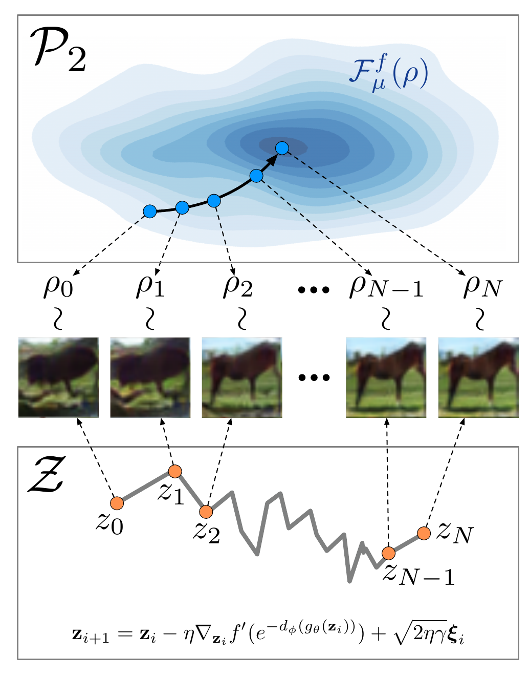Figure 1:  An illustration of refinement using DGflow, with the gradient flow in the 2-Wasserstein space P2 (top) and the corresponding discretized SDE in the latent space (bottom). The image samples from the densities along the gradient flow are shown in the middle. From [1] - Figure 1     

Refining the latent results in better quality generated image. In practice, the final algorithm looks as follows.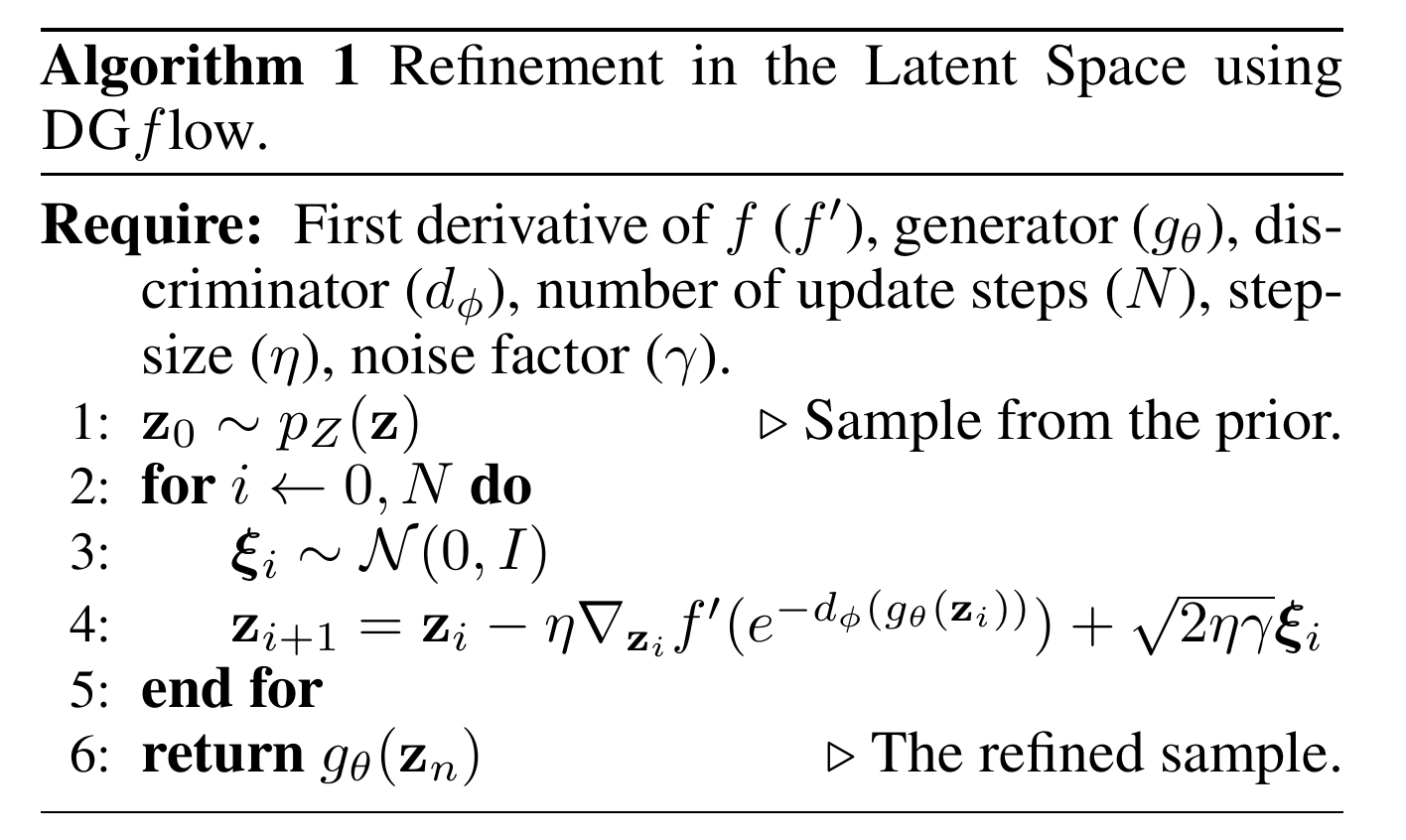We can also extend this approach to the case of vector-valued discriminators as well as VAEs and Normalising flows.

Results

The paper presented empirical results for various deep generative models with the goals of determining DG flow's effectiveness at improving samples produced by the generator, and showing its flexibility at working for different types of models, data, and metrics. Achieving state-of-the-art results compared to existing generators was not the goal of the experiments, but instead to demonstrate DG flow's ability to improve generated samples compared to the bare estimators. The experiments were run for three different f-divergences; Kullback-Leibler (KL), Jensen-Shannon (JS), and $$log\;D$$ divergences [14]. DG flow is shown to outperform the base model in both the synthetic and image-based datasets. This demonstrates DG flow's effectiveness at improving samples from generative models.

Synthetic Dataset Experiments

The datasets used to run the experiments were 5000 samples from each of the synthetic 25Gaussians and 2DSwissroll datasets. These simple datasets provide a straightforward way of visually inspecting results by plotting the generated samples on top of the true distribution. Varying the time-steps for the generated samples illustrates the nature of the generated samples converging (or not) to the true distribution. 5000 samples were generated from a trained Wasserstein GAN with gradient penalty (WGAN-GP) [15], and were then refined using DG flow for each of the datasets.

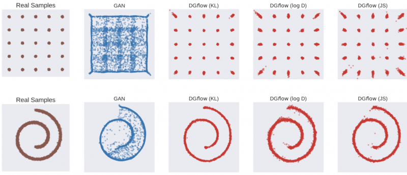Figure 2: Comparison of the true distribution (brown) of the synthetic datasets (25Gaussians on top, 2DSwissroll on bottom) with samples generated using the WGAN-GP (blue) and WGAN-GP refined with DG flow using KL, $$log\;D$$, and JS divergences respectively (red).

Figure 2 shows the plotted points from the synthetic datasets (25Gaussians on top, 2DSwissroll on bottom) for the original true distribution of data (brown), samples generated using the WGAN-GP (blue), and samples generated using WGAN-GP refined with DG flow with KL, $$log \;D$$ and JS divergences respectively (red). For both datasets, it is clear that the generator refined with DG flow approximates the true distribution significantly better, recovering the correct structure of data. DG flow with KL for the f-divergence approximates the true distribution the best.

A quantitative comparison was also made for the 25Gaussians dataset using the percentage of high-quality samples and the kernel density (KDE) score as the qualifying metrics. A sample is deemed to be of high quality if it lies within four standard deviations of its nearest Gaussian. The KDE score is used to estimate the probability density function of a random function by using generated samples to estimate the KDE and then computing the log-likelihood of the true samples using the KDE estimate. For more on the KDE, see this quick interactive tutorial. This gives us a measure of distance of the generated distribution from the true distribution. The results of these metrics applied to the base WGAN-GP and the DG flow refined generators are shown in Table 1. Each of the DG flow refinement implementations outperforms the base WGAN-GP generator. The DG flow using KL divergences has the best score in both the percentage high quality and KDE score metrics. This agrees with the qualitative comparison above where KL was shown to be the best divergence method for this experiment.

Table 1: Quantitative comparison of different generator methods on 25Gaussins dataset. Higher percentage quality and lower KDE scores are better. The best scores are highlighted in bold.

Image Dataset Experiments

Experiments were run using the CIFAR10 image dataset to test how effective DG flow is with real-world image datasets. Instead of using the Inception Score (IS) [16] alone, the Fréchet Inception Distance (FID) [17] was also used to evaluate image quality. IS works by quantifying how well the Inception v3 image classifier classifies synthetic (in this case, generated) images into one of one thousand of CIFAR10 classifications to estimate the quality of the generated images. This metric combines the quality (confidence of the class predictions) and the diversity (integral of the marginal probability of the class predictions) of the generated images. However, IS does not compare the generated images to the ground truth images. Instead, we use FID to account for this. FID compares statistics of the ground truth images to the statistics of the generated images to form a measure of distance. For more on IS and FID, see this tutorial.

WGAN-GP and SNGAN [18] with a RESNET backbone (SN-ResNet-GAN), which use scalar-valued discriminators were used as base models, and DG flow was applied to each of these models for each of the three f-divergence methods (KL. $$log \;D$$ and JS). The table of empirical results is shown in Table 2 for FID. Lower FID scores are better. These results show all DG flow methods outperform the base models for image data. The JS f-divergence has the best FID score for the WGAN-GP model, and the KL f-divergence gave the best score for the SN-ResNet-GAN model.

Table 2: Quantitative comparison of different generator methods on the CIFAR10 image dataset. Lower scores are better. The best scores for each model are highlighted in bold.

References

[1] Goodfellow, I. J. et al. Generative Adversarial Networks. arXiv:1406.2661 [cs, stat] (2014).

[2] Azadi, S., Olsson, C., Darrell, T., Goodfellow, I. & Odena, A. Discriminator Rejection Sampling. arXiv:1810.06758 [cs, stat] (2019).

[3] Turner, R., Hung, J., Frank, E., Saatci, Y. & Yosinski, J. Metropolis-Hastings Generative Adversarial Networks. arXiv:1811.11357 [cs, stat] (2019).

[4] Tanaka, A. Discriminator optimal transport. in Advances in Neural Information Processing Systems vol. 32 (Curran Associates, Inc., 2019).

[5] Che, T. et al. Your GAN is Secretly an Energy-based Model and You Should Use Discriminator Driven Latent Sampling. in Advances in Neural Information Processing Systems vol. 33 12275–12287 (Curran Associates, Inc., 2020).

[6] Gulrajani, Ishaan, et al. "Improved training of Wasserstein gans." arXiv preprint arXiv:1704.00028 (2017).

[7] Santambrogio, Filippo. "{Euclidean, metric, and Wasserstein} gradient flows: an overview." Bulletin of Mathematical Sciences 7.1 (2017): 87-154.

[8] Arjovsky, M., Chintala, S. & Bottou, L. Wasserstein Generative Adversarial Networks. in International Conference on Machine Learning 214–223 (PMLR, 2017).

[9] Liu, D., Vu, M. T., Chatterjee, S. & Rasmussen, L. K. Entropy-regularized Optimal Transport Generative Models. ICASSP 2019 - 2019 IEEE International Conference on Acoustics, Speech and Signal Processing (ICASSP) 3532–3536 (2019) doi:10.1109/ICASSP.2019.8682721.

[10] Ansari, A. F., Ang, M. L. & Soh, H. Refining Deep Generative Models via Discriminator Gradient Flow. arXiv:2012.00780 [cs, stat] (2021).

[11] Risken, H. & Frank, T. The Fokker-Planck Equation: Methods of Solution and Applications. (Springer-Verlag, 1996). doi:10.1007/978-3-642-61544-3.

[12] Beyn, W.-J. & Kruse, . Numerical methods for stochastic processes. Lecture Book (in preparation).

[13] Sugiyama, M., Suzuki, T. & Kanamori, T. Density Ratio Estimation in Machine Learning. (Cambridge University Press, 2012).

[14] Gao, Y. et al. Deep Generative Learning via Variational Gradient Flw. in International Conference on Machine Learning 2093–2101 (PMLR, 2019).

[15] Gulrajani, I., Ahmed, F., Arjovsky, M., Dumoulin, V. & Courville, A. C. Improved Training of Wassers

[16] Salimans, T. et al. Improved Techniques for Training GANs. in Advances in Neural Information Processing Systems vol. 29 (Curran Associates, Inc., 2016).

[17] Heusel, M., Ramsauer, H., Unterthiner, T., Nessler, B. & Hochreiter, S. GANs Trained by a Two Time-Scale Update Rule Converge to a Local Nash Equilibrium. in Advances in Neural Information Processing Systems vol. 30 (Curran Associates, Inc., 2017).

[18] Miyato, T., Kataoka, T., Koyama, M. & Yoshida, Y. Spectral Normalization for Generative Adversarial Networks. arXiv:1802.05957 [cs, stat] (2018).