The supreme goal of all theory is to make the irreducible basic elements as simple and as few as possible without having to surrender the adequate representation of a single datum of experience.

Albert Einstein, 1933

In today's world, deep learning has found applications within a myriad of different tasks and can be found in most high-end software products. However, most workstations that power or train such systems contain expensive, large, and power-hungry graphical processing units (GPUs), most often powered by the parallel computing platform CUDA. But in this age, smaller "smart" devices, such as mobile phones, TVs, cars and even doorbells may also find utility in the solutions offered by such deep-learning models in e.g. computer vision and are therefore inevitable deployment targets of such solutions. However, how can devices with limited cooling, power and computational capabilities run large complex neural networks? The short answer is they couldn't, however, the solution has been in the making for decades and involves immense hardware progress, software innovation and neural network optimisations. As of this writing, the compute capability of a high-end phone's neural network engine, such as the iPhone 12 Pro Max, is comparable to that of a mid-range GPU from a few years ago.

In this blog, we will look at a method of producing state of the art neural networks for edge devices. Specifically at a method of obtaining hardware-aware efficient neural networks. [0] provides an overview of the current state of deep learning model execution on mobile phones until September 2018, in terms of mobile architectures and hardware.

Introduction

It should appear intuitive that smaller networks, with less, compute and memory requirements are better suited for edge devices. There are many examples of modified operators and architectural changes proposed in the last few years, in an effort to make the network more compute-efficient. Examples of such models are MobileNet (V1, V2), ShuffleNet (V1, V2), EfficientNet (V1, V2), ShuffleNet (V1, V2). Most of these models, while small, start from the assumption that if a small "mobile-runnable" network is what is needed, then training a small "mobile-runnable" network is the route of choice. There is an orthogonal line of thinking, perhaps counterintuitive, that instead states that a smaller more efficient model is best obtained by starting with a larger model and reducing its size. One way of gaining an intuition for this approach is to do the counterintuitive, and view an initialized neural network training as a lottery.

Imagine a lottery where the lottery price is a neural network with high accuracy, and the tickets are subnetworks of a larger network that contains p % of the larger networks weights, you win if the smaller network (lottery ticket) obtains comparable performance to the larger network. Would you expect there to be winning tickets for subnetworks that are much smaller than the large network—yet yield approximately the same performance in fewer or the same training iterations?

The lottery ticket hypothesis in [7],  postulates and provides empirical evidence for the hypothesis that there exist subnetworks within any large, dense network that can obtain approximately the same performance, for the vision tasks considered. By method of pruning or sparsification it is postulated that it is possible to identify such subnetworks (referred to as winning tickets within this lottery) for which the following holds: in less than or equal training time, the subnetwork achieves equal or better loss with much fewer parameters.

In the paper the authors run a number of small vision experiments for convolutional networks and identify smaller subnetworks that when trained in isolation reach comparable performance to the larger dense network from which the subnetwork was derived, such winning tickets may have orders of magnitude fewer parameters and computational constraints. An interesting observation made in the paper is that reinitializing the subnetwork leads to worse performance compared to using the initialization of weights as part of the initialization of the larger network. In brief, the method used in the paper is that of iterative pruning:

1. The network is randomly initialized

2. The network is trained for some number of iterations

3. Prune $$p^{(1/n)} %$$ of the smallest magnitude weights

4. Repeat step 1 to 3 $$n$$ times

Another hypothesis of the paper is that larger networks are easier to train than smaller networks since there are many possible winning tickets in a larger network. However, notably, the experiments were carried out for small vision datasets, and the network uncovered in the paper were not optimized for modern hardware.

In addition, a key issue with the method above is the fact that runtime constraints such as latency, energy usage, or memory usage on the edge device are not accounted for during the network construction of any of the subnetworks. In the ideal case, the convolutional network design should be hardware-aware and efficient for the particular edge device hardware.

In the paper "FBNet: Hardware-Aware Efficient ConvNet Design via Differentiable Neural Architecture Search" an efficient differentiable neural architecture search (NAS) framework is presented that is able to produce a distribution of architectures that is optimized based on hardware latency.

FBNet: Hardware-Aware Efficient ConvNet Design via Differentiable Neural Architecture Search

As mentioned in the introduction, the process of designing an efficient convolutional network is a difficult task. Made even more difficult when the network design must be optimised for some particular hardware. In the paper, the authors highlight 3 main issues.

Intractable design space

Taking the example of a relatively small network such as VGG16. Say that the kernel size could take on the values $${{1,3,5}}$$ and filters $$ {32,64,128,256,512}$$, the possible combinations for the network are then $$(3 \cdot 5)^{16} \approx 6 \cdot 10 ^{18}$$ possible architectures. Training any such architecture to judge its performance might take days or weeks; as a result, training time is commonly limited.

A method of reducing the intractable cost to a reduced, yet still prohibitively high, is to use reinforcement learning to select suitable architectures. The way this has been done before is by using a controller that generates architectures from a search space, which are then trained. The cost of this approach is still high since thousands of networks must still be trained. To reduce training time it is common to use proxy datasets or train for fewer epochs.

Nontransferable optimality

The authors argue that different hardware has different optimality in terms of architecture and that estimated FLOP counts are poor indicators of latency on any particular hardware. This is because the latency or energy usage of an operation empirically vary for different hardware by at least 40%.

The Problem of Hardware-agnostic Metrics

Most previous works use hardware-agnostics metrics such as floating-point operations (FLOPs)—in reality, the number of multiply-add operations for some layers—to estimate the efficiency of the network. But based on other research, this may be a poor indicator, e.g. NasNet-A [2] has a similar FLOP estimation to MobileNetV1, but the design is not hardware friendly, so the latency is larger, by over 20% [3]. This is due to the interconnectivity introduced in the blocks produced by NAS, which increases memory movement. This is something we also observed at Deep Render when working with NAS early on. 

Proposed Method

To address the problems above, in obtaining hardware-aware efficient neural networks, the authors propose the scheme seen below.

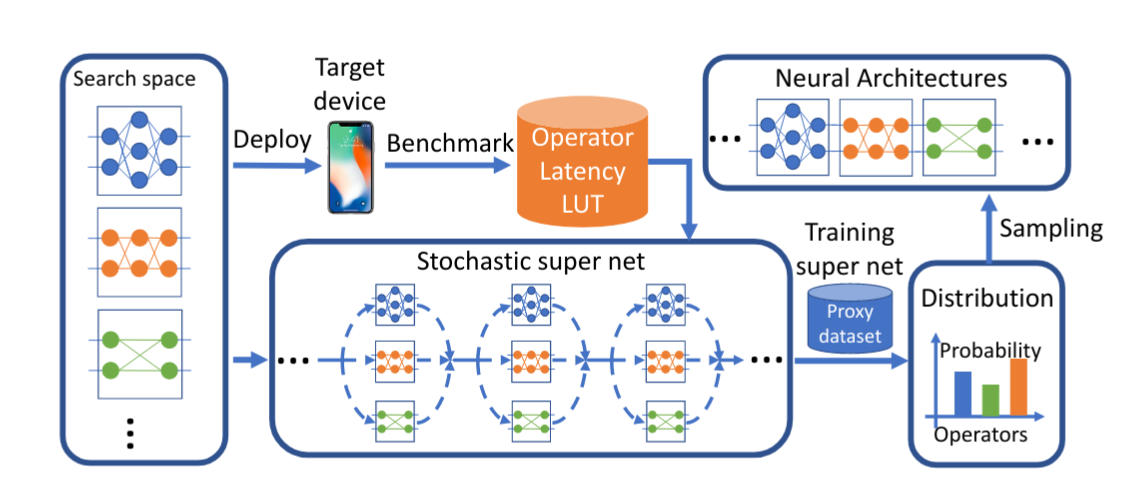Figure 1: The proposed Facebook-Berkley-Nets (FBNet) approach to hardware-aware efficient network design. Taken from [1].

In the figure above an overview of the FBNet framework is seen.  It is a differentiable neural network architecture search (NAS) scheme to find hardware-aware efficient convolutional neural networks (ConvNets). In the following section, we will discuss how it works.

The Loss Function

The architecture search problem is formulated as follows:

$$ min_{a \in A} min_{w_a} L(a, w_{a}) $$

where the goal is to find an architecture $$a$$, part of the architecture search space $$A$$, that achieves the lowest loss $$L$$. The loss function that is selected is latency-aware, and is defined as follows:

$$ L(a, w_{a}) = L(a, w_{a}) + \alpha * log(LATENCY(a))^\beta$$.

The first term $$L$$ denotes the network training objective. In the paper the authors searched for architectures for object detection or classification, as such, cross-entropy was chosen as a loss, meaning $$L = CE(a, w_{a})$$. In general, $$L$$ would be the standard loss used before the training became hardware-aware. $$\alpha$$ controls the importance of the latency constraint in the new loss, whereas $$\beta$$ modulates the magnitude of the latency in the loss. The second term, $$LATENCY(a)$$ denotes the hardware latency of the architecture $$a$$.

Given that the search space of possible architectures includes $$10^{21}$$ architectures, how did the authors compute the latency for each architecture? It turns out that they didn't.  Estimating the latency of $$10^{21}$$ architectures would be intractable, even for Facebook. Since the number of architectures scales exponentially as $$O (\# ops^{\# layers})$$, the authors propose a method of transforming the complexity from $$O (\# ops^{\# layers})$$ to $$O (\# ops \cdot \# layers)$$. This is done via an approximation of the latency for each architecture $$a$$, computed as the sum of the latency of all blocks $$b_{i}^{a}$$. For all hardware, for which a ConvNet should be produced, the latency of every block available to the NAS was computed, on the hardware. Using this data, a look-up table was used to quickly estimate the total latency $$LATENCY(a)$$ as

$$LATENCY(a) = \sum_{i} LATENCY(b_{i}^{a})$$

where $$b_{i}^{a}$$ denotes a particular layer or block at index $$i$$ in the network for architecture $$a$$. It is important to note that this only holds if the runtime of each operation on the target hardware is independent of other operations. Unfortunately, no empirical evidence is provided to justify this claim by the authors. However, since the latency for each operator is a constant coefficient, the overall total loss is fully differentiable. We would like to see a small follow-up study in the future that reaffirms this belief.

The Search Algorithm

As opposed to earlier papers that mainly employ a cell level architecture search, which is impractical for mobile CPUs (due to the complex branches that often result), the authors use a layer-wise search space, with fixed macro-architecture. This means that the overall network structure is fixed to $$n$$ layers, but the operations within each layer will be learnt. To do this, the authors represent the search space by a so-called "stochastic supernet".  The supernet is a probabilistic network that contains one computational block at each level stochastically, i.e. each block has a sampling probability of being picked, $$\theta_{l}$$.

At each layer, a block is sampled based on the associated sampling probability for the layer $$\theta_{l}$$. This process of a stochastic super net is shown in the diagram, and the sampling function is shown below.

$$ P_{\theta_{l}} (b_{l} = b_{l,i})  = softmax(\theta_{l,i} ; {\theta_{l}}) = \frac{e^{(\theta_{l,i})}}{\sum_{i} e^{\theta_{l,i}}} $$

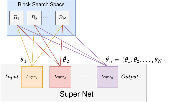Figure 2: An example of a probabilistic supernet with weights $$\hat{\theta}_{l}$$, along with a block search space containing blocks $$\{B_{1}, B_{2}, ..., B_{N}\}$$. These blocks contain some number of computational units internally such as convolutional layers and activations that are executed as part of some layer. For the case of the FBNet paper, only 1 block is sampled for each layer $$l$$, based on the softmax probability of $$\hat{\theta}_{l}$$. Performing this sampling for every single layer will then yield an architecture $$a \in A$$. 

An equivalent way of viewing the sample operation, is as if a mask is applied on the candidate blocks for each layer, where the output of the next layer $$l+1, x_{l+1}$$ can be expressed as

$$x_{l+1} = \sum_{i} m_{l,i} \cdot b_{l,i}(x_{l})$$

where $$i$$ is the index into the candidate block used at layer $$l$$. $$m_{l,i}$$ is a binary mask in $$\{0,1\}$$. That is, if $$m_{l,i}$$ is $$0$$, then the block candidate at layer $$l$$ with index $$i$$ will be ignored. In the paper the authors sample each layer independently, as such, the probability of any one architecture $$a \in A$$ is

$$P_{\theta} = \prod_{l} P_{\theta_{l}}(b_{l}=b_{l,i}^{a})$$

Careful readers might spot a potential issue with the sampling methods discussed above. The problem is that the search space is discrete, whereas gradient descent-based methods prefer continuous spaces. How do we train the super net if we use discrete sampling since it will not allow gradients to flow back into the $$\theta$$ parameter? Whenever there is an issue of discreteness within neural network training a common tactic is to try to relax the process.

Imagine that instead of having a hard binary max switch that could only take on the values $$\{1,2\}$$ (i.e. we can only sample discrete states), is there a differentiable approximation of sampling discrete data we could use to relax the sampling problem? As is common, someone else has already solved the problem for us. Gumbel SoftMax is a modification to the softmax function shown above, that adds a temperature parameter [4]. This allows the authors to relax the discrete mask $$m_{l,i}$$ into a continuous random variable. The Gumbel Softmax function is defined as follows

$$GumbelSoftmax(\theta_{l,i}|\theta_{l}) = \frac{e^{(\theta_{l,i}+g_{l,i})/\tau}}{\sum_{i} e^{(\theta_{l,i}+g_{l,i})/\tau}}$$

where $$g_{l,i}$$ sampled from $$Gumbel(0,1)$$ is random noise that follows the Gumbel distribution. This variation of the softmax function is controlled by the new temperature parameter $$\tau$$. As $$\tau$$ approaches 0, we approach a discrete sampling process, whereas when $$\tau$$ becomes large, $$m_{l,i}$$ becomes a continuous random variable. For an overview of the Gumbel trick that was applied here, [5] provides a great explanation.

Finally, if you look back at the loss we started with

$$min_{a \in A} min_{w_a} L(a, w_{a})$$

we can now re-write this for a continuous case

$$min_{\theta} min_{w_a} E_{a ~ P_{\theta}} L(a, w_{a})$$

The loss above is fully differentiable since it is differentiable with respect to the network weights $$w_{a}$$ and after applying the Gumbel trick to relax the softmax sampling function, we can now get gradients for the sampling parameter $$\theta$$, since gradients can pass through the now continuous sampling process. Given that the loss is now fully differentiable, how do they actually train this super net?

Training

During training, $$\frac{\partial L}{\partial w_{a}}$$ is computed to train the weights in each layer of the super net. This is the same as training an ordinary network. After the operator weights have been trained they will have a different impact on the accuracy of the network. Therefore $$\frac{\partial L}{\partial \theta}$$ is computed to update the sampling probability $$P_{0}$$ for each block, which select operators with the optimal accuracy and latency trade-off for the given balance of the terms in the loss function $$L$$. Finally, once the training is finished, the cool thing is that we can just grab samples from $$P_{0}$$ to produce different architectures $$a \in A$$, that satisfy the latency requirement.

Finally to give some context into how the training was actually executed. In more practical terms, the method by which the super net was trained was by using 100 ImageNet classes—they refer to this as a proxy dataset. In one epoch, they first trained the operator parameters $$w_{a}$$ on $$80\%$$ of the training set using stochastic gradient descent with momentum. Following this, the remaining $$20\%$$ of the epoch was used to learn the architecture distribution parameters $$\theta$$, with an Adam optimizer. The split training of the weight and architecture parameters helped to ensure generalization on the validation dataset. Finally, the researchers found that for training stability and to avoid an architecture collapse, where only the cheapest operators would become selected (because each operator's importance to the accuracy at the start is unclear), they decided to

"[...] postpone the training of the architecture parameter θ by 10 epochs to allow operator weights to be sufficiently trained first".

This means that for the first 10 epochs, each block is sampled with equal probability and for every iteration, a different convolutional neural network is constructed and trained (you could imagine this as a particular instantiation of the super net). This ensures that every block, for each layer, in the search space is trained, such that after 10 epochs, the addition of the latency loss will not result in just the fastest operations being considered, since each block's impact on the accuracy will be more clear following the pre-training.

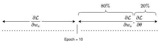Figure 3: Overview of the training scheme of FBNet. For the first $$10$$ epochs only $$\frac{\partial L}{\partial w_{a}}$$ is computed. After $$10$$ epochs, $$80\%$$ of the epoch is used to train the sampled block weights using $$\frac{\partial L}{\partial w_{a}}$$, the remaining $$20\%$$ is used to train the sampling weights $$\frac{\partial L}{\partial \theta}$$. 

Results

In this blog post, we did not find it interesting to discuss the results in detail. However it is worth highlighting that the FBNet approach is substantially more efficient than any other approach, yielding networks of better or similar accuracy in orders of magnitude less GPU compute time. As an example, the paper "MnasNet: Platform-Aware Neural Architecture Search for Mobile" [6], takes about 400 times more GPU hours to find a network of similar quality. For other NAS based approaches, they estimate about 200 times more GPU hours.

Another interesting aspect of the results to mention is that the authors highlight clear device latency differences, to justify the complexity of training hardware-aware convolutional neural networks.

Hardware-aware Awareness

The authors apply the FBNet to generate models adapted for iPhone X and Samsung S8 hardware. Notably, using the network that was trained for the iPhone X on the Samsung S8 resulted in an increased latency of about 18 %, whereas taking the Samsung S8 optimized network and deploying it on the iPhone X resulted in about 40 % increased latency. This result of cross-deployment of models is summarised in the table below [1]:

Table 1: Overview of the 2 hardware models trained, and latency of cross deployment.

The authors suggest that hardware differences cause some computational blocks to be more efficient on the iPhone X or the Samsung S8. As an example, they provide operator runtimes on the iPhone X and the Samsung S8 devices for depthwise convolutions, shown in the figure below, which is used to suggest why the iPhone X model performs so much worse when run on the Samsung S8 device.

Whilst far from a complete study, these results indicate that for optimal mobile deployment, considering the hardware of the target device is important.

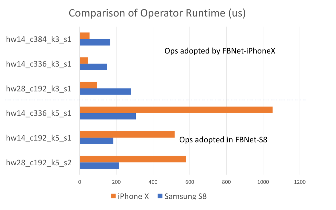Figure 4: Depthwise convolutional operator benchmarks from the FBNet paper for iPhone X and Samsung S8. Some operators are much faster on the Samsung S8 device compared to the iPhone X device. Taken from [1]. 

Conclusion

In this blog post, we discussed the novel hardware-aware neural architecture search approach in [1], that yields mobile models in several orders of magnitude fewer GPU hours compared to other methods, and in addition, is built to take hardware into consideration. A key reason behind the hardware-aware training is the notion that any type of FLOP or compute cost metric is inexact and hardware agnostic, this was shown to lead to significant performance differences for different hardware even if the FLOPs or parameters are almost the same.

Appendix

Implementation

In this section, a brief summary of the practical implementations of the paper will be provided. It is of less interest since the theoretical discussion in the other sections is deemed more useful in actually understanding the process and training your own super net.

Hyperparameters

In the loss function, $$\alpha$$ was set to $$0.2$$, $$\beta$$ to $$0.6$$ and the temperature in the Gumbel Softmax was to to $$5.0$$ and then annealed by $$e^{-0.045} \approx 0.956$$ every epoch.

Block Search Space

For the block search space that is depicted in figure 2, there are 9 blocks available as part of the FBNet search space, detailed in the table below. Kernel indicates the convolutional kernel size. Groups the number of groups of filters in the convolution, and Expansion refers to how much the first 1x1 convolution is expanded compared with its input channel size.

Table 2: Available block types for FBNet.

The Macro Architecture

Input Shape ($$[C,H,W]$$)	Block	# Filters	# Blocks	Stride of First Block
$$[3,224,224]$$	3x3 Conv	16	1	2
$$[16,112,112]$$	TBD	16	1	1
$$[24,56,56]$$	TBD	24	4	2
$$[32,28,28]$$	TBD	32	4	2
$$[64,14,14]$$	TBD	112	4	2
$$[112, 14, 14]$$	TBD	184	4	1
$$[184, 7, 7]$$	TBD	352	1	2
$$[352, 7, 7]$$	1x1 Conv	1504	1	1
$$[1504, 7 ,7]$$	7x7 AvgPool	1504	1	1
$$[1504]$$	Fully Connected	-	1	-

Table 3: The macro architecture of FBNet.

In the table above, the fixed macro architecture of FBNet can be seen, where "TBD" refers to a block type that will be determined by the training and sampled during inference from $$P_{\theta}$$ based on the available block types in Table 2.

In total, the architecture of the paper contains 22 layers, which can each choose from 9 possible blocks, which gives $$9^{22} \approx 10^{21}$$ possible architectures.

Sources

[0] Andrey Ignatov, Radu Timofte, Andrei Kulik, Seungsoo Yang, Ke Wang, Felix Baum, Max Wu, Lirong Xu, Luc Van Gool: “AI Benchmark: All About Deep Learning on Smartphones in 2019”, 2019; [http://arxiv.org/abs/1910.06663 arXiv:1910.06663].

[1] Bichen Wu, Xiaoliang Dai, Peizhao Zhang, Yanghan Wang, Fei Sun, Yiming Wu, Yuandong Tian, Peter Vajda, Yangqing Jia, Kurt Keutzer: “FBNet: Hardware-Aware Efficient ConvNet Design via Differentiable Neural Architecture Search”, 2018; [http://arxiv.org/abs/1812.03443 arXiv:1812.03443].

[2] B. Zoph, V. Vasudevan, J. Shlens, and Q. V. Le. Learning transferable architectures for scalable image recognition.arXiv preprint arXiv:1707.07012, 2(6), 2017

[3] M. Sandler, A. Howard, M. Zhu, A. Zhmoginov, and L.-C.Chen. Mobilenetv2: Inverted residuals and linear bottle-necks. InProceedings of the IEEE Conference on ComputerVision and Pattern Recognition, pages 4510–4520, 2018.

[4] E. Jang, S. Gu, and B. Poole. Categorical parameterization with gumbel-softmax.arXiv preprint arXiv:1611.01144,2016.

[5] https://sassafras13.github.io/GumbelSoftmax/

[6] Mingxing Tan, Bo Chen, Ruoming Pang, Vijay Vasudevan, Mark Sandler, Andrew Howard, Quoc V. Le: “MnasNet: Platform-Aware Neural Architecture Search for Mobile”, 2018, CVPR 2019; [http://arxiv.org/abs/1807.11626 arXiv:1807.11626].

[7] Jonathan Frankle, Michael Carbin: “The Lottery Ticket Hypothesis: Finding Sparse, Trainable Neural Networks”, 2018, ICLR 2019; [http://arxiv.org/abs/1803.03635 arXiv:1803.03635].