Introduction

In terms of generative adversarial networks (GANs) for image generation, the StyleGAN 2 network has for a long time been considered state-of-the-art, or close to it, for various image generation tasks. Looking at the images produced by the network, it's apparent that it's able to produce realistic-looking images, and a lot of research papers have suggested improvements to lower the FID score. However, within the large family of GANs for image and video generation that spawned e.g. StyleGAN 2, a massive overlooked issue has for a long time remained unsolved. This issue can best be seen when we visualize temporal generation such as generated video or latent space exploration as in the videos below.

In the 2 videos above, as we traverse the latent space, textures appear to "stick" to pixel locations of the image. The authors of the paper Alias-Free GAN (Karras et al.) state the observed issue above as follows:

the synthesis process of typical generative adversarial networks depends on absolute pixel coordinates in an unhealthy manner. This manifests itself as, e.g., detail appearing to be glued to image coordinates instead of the surfaces of depicted objects

The paper suggests that this phenomenon occurs because most GAN architectures suffer from aliasing. They argue that aliasing results in an information leak within the network causing dependence on absolute pixel locations, causing the texture-sticking effect. Following the author's adjustments to the network operations, along with a few other tweaks, they are able to achieve the following results.

Notice in the videos above that the textures no longer stick to a particular pixel location, and instead naturally follow the object in the scene. In this blog post we will answer why this is the case, and explain:

• Aliasing from a signal processing perspective
  
  
• The concept of equivariance
  
  
• What it means for a GAN to suffer from aliasing
  
  
• How the authors modified the StyleGAN 2 to remove texture-sticking
  
  
• Possible relevance to AI-based compression

Finally, what do these neon-aliens have to do with it?

But first, some background:

Unintended Positional Encoding in CNN's

The texture sticking in the linked videos is striking, but what does this have to do with aliasing?

Naively:

• We roughly think of CNNs operating hierarchically, with "coarse" features corresponding to earlier layers and "fine" features being learned by later layers. This mental model seems to be violated when the fine features of a person's beard are fixed in position while the coarse features move around in latent space exploration.
  
  
• Aliasing is when two signals cannot be distinguished from one another, because the data is not sampled frequently enough. This can cause artifacts if we use the wrong signal, which was indistinguishable from the correct signal.

The connection between these two ideas has been built up in a lot of the surrounding literature and is explained in this key paragraph from the Alias-Free GAN paper:

It turns out that current networks can partially bypass the ideal hierarchical construction by drawing on unintentional positional references available to the intermediate layers through image borders [27, 34, 63], per-pixel noise inputs [32] and positional encodings, and aliasing [5, 65]. Aliasing, despite being a subtle and critical issue [43], has received little attention in the GAN literature. We identify two sources for it: first, faint after-images of the pixel grid resulting from non-ideal upsampling filters (e.g., nearest, bilinear, strided convolutions), and second, the pointwise application of nonlinearities such as ReLU. We find that the network has the means and motivation to amplify even the slightest amount of aliasing and combining it over multiple scales allows it to build a basis for texture motifs that are fixed in screen coordinates. This holds for all filters commonly used in deep learning [65, 57], and even high-quality filters used in image processing.

Summarising: aliasing (among other things) causes unintended positional encoding to be used by the network and this causes the observed texture sticking. As always, if the network can find a way to "cheat," it does!

We highlight papers mentioned by the authors that we think you may find most interesting:

• (2019) Making Convolutional Networks Shift-Invariant Again
  
  
• (2019) Why do deep convolutional networks generalize so poorly to small image transformations?

Both of these papers focus on the observations that CNN classification performance sometimes changes drastically when input images images are perturbed slightly:

This is surprising given that this should not happen if CNNs are translation-invariant, and in addition, these networks are supposed to be robust to input perturbation by training with data augmentation.

This leads Karras et al. to make the following string of arguments:

• Texture sticking in the latent space is caused by unintended positional encoding
  
  
• The most difficult obstacle to eliminating the unintended positional encoding is aliasing
  
  
• Aliasing is most easily solved from a classical signal processing perspective, which views image pixels as discrete samples of some underlying continuous signal
  
  
• Then removing unintended positional encoding is equivalent to translation (and optionally rotation) equivariance on the underlying continuous signal

Let's review aliasing and some signal processing, so that we can build out these arguments.

Signal Processing - Aliasing

Aliasing is when two different signals cannot be distinguished from one another (they are aliases of each other), because the data is not sampled frequently enough. This can cause artifacts if we use the wrong signal, which was indistinguishable from the correct signal.

How frequently do we need to sample our data to avoid aliasing? The Nyquist–Shannon sampling theorem gives a simple answer:

Consider a signal $$x(t)$$. Via the Fourier transform, we can think of it as being composed of a (possibly infinite) number of signals of various frequencies. If the highest of these frequencies is $$\frac f2$$ then we can guarantee no aliasing (the signal is uniquely determined) if we sample the data more frequently than $$f$$.

Said another way:

Suppose we sample our data at frequency $$f$$. Then we can perfectly reconstruct the original signal (no aliasing) if all underlying frequencies in the original signal $$x(t)$$ are less than $$\frac f2$$. The frequency $$\frac f2$$ is known as the Nyquist frequency.

Aliasing doesn't just occur for time-dependent signals, it can occur anytime you are periodically sampling some continuous function.

For example, an image on your computer screen is a 2D array of discrete samples (pixels) of some real world continuous signal. The Nyquist–Shannon sampling theorem says that if you have too low a spatial sampling rate ie. too low resolution, the true signal is not guaranteed to be represented accurately.

The most familiar case of spatial aliasing is when curved lines and edges have a pixelated "staircase" pattern at low resolution:

Spatial aliasing can also create interesting artifacts, such as the warping of high frequency parts of the image seen below:

Source: http://mielliott.github.io/index.html

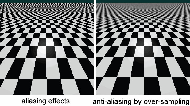
The sampling theorem tells us that we can correct poor signal representation and aliasing artifacts by sampling more frequently (increasing image resolution). However, in practice we typically have a fixed resolution and seek to correct aliasing via some other method. In this case, various strategies are used:

• Convolve (equivalent to multiplying in the frequency domain) the image with a filter that reduces high frequency information. Example: gaussian blur.
  
  
• Increase sampling in important regions of the image/video

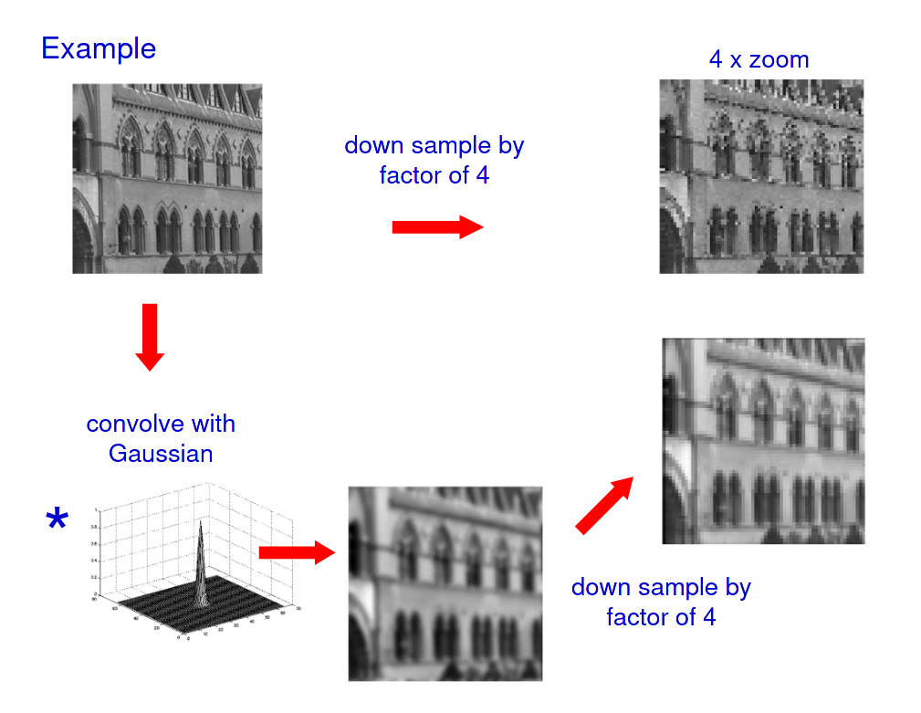Convolving with a gaussian is equivalent to multiplying by a gaussian in the frequency domain. This greatly reduces higher frequencies (low pass filter), making for better visual quality at low resolutions.
Source: https://www.robots.ox.ac.uk/~az/lectures/ia/lect2.pdf

Aside: Anti-aliasing in your favourite video games carries out some advanced extensions of these ideas! The practical goal is to come up with algorithms that reduce aliasing for lower compute than the cost of increasing image/video resolution.

Now that we understand aliasing, how do the authors remove it from GANs?

A recipe for equivariant GANs

Neural networks can be constructed in any number of ways, however typically the building blocks for generative adversarial networks are limited to only a few basic operations. In the paper, the authors consider the following operations:

• Convolutions
  
  
• Upsampling & Downsampling
  
  
• (Pointwise) Nonlinearities

and demonstrate mathematically how each operation may fail to satisfy equivariance, or lead to aliasing. It is these two different concepts that the authors attribute to the texture-sticking effect; due to the injection of unwanted side information. Before we discuss what is wrong with the current operations and how we can fix them, we will briefly discuss equivariance.

Equivariance is a mathematical concept from group theory. We are interested in 2 particular types of equivariance: translation and rotation. Firstly, equivariant to translation means that a translation of input features results in an equivalent translation of the outputs. Similarly, equivariant to rotation means that a rotation of input features results in an equivalent rotation of the outputs. See GIFs below for an example involving CNN feature maps.

Equivariance may also be expressed mathematically as:

$$f(g(x)) = g\;'(f(x))$$

and shown as a diagram between two domains below:

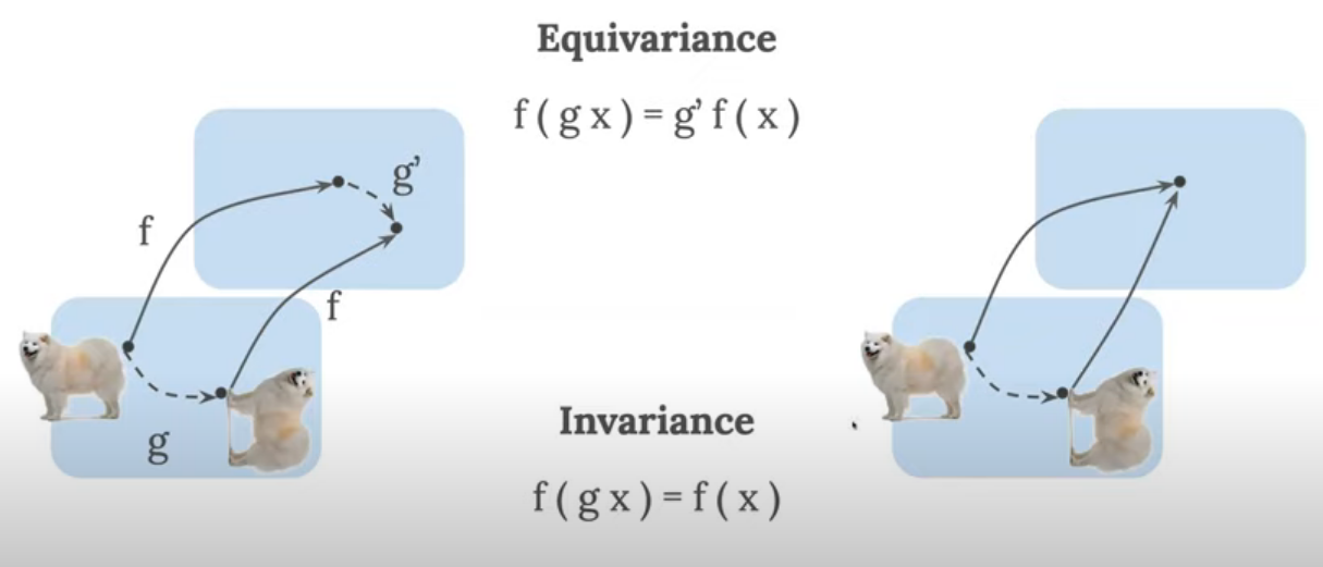Left: equivariance example where normal and rotated dog maps to different locations in the other domain. Right: the normal and rotated dog maps to the same location (e.g. same label). Source: https://www.youtube.com/watch?v=03MbWVlbefM&t=1393s

As a side note, the case of invariance is useful in e.g. supervised learning tasks, where the rotation of the dog should not alter the label assigned, however, for image generation it is clearly unwanted.

How to measure equivariance?

Based on the description of translation and rotation equivariance above, a method of quantifying equivariance is to do the following:

• Apply transformation $$t$$ to transform the input noise $$n$$, send it to the generator and produce image $$Img_{t}$$
• Take input noise $$n$$, send it to the generator to produce image $$Img$$, apply $$t$$ onto $$Img$$

Given these 2 images, the authors compute a PSNR that estimates the equivariance in terms of dB:

$$EQ_{T} = 10 \cdot log_{10} \cdot {I_{max}^2 \over (Img_{t} - t(Img))^2}$$

For the case of rotation equivariance, discretely sampled images are not radially symmetric and so the computation is a bit more involved, but for this blog, the description above suffices. In Appendix section E.3 the equivariance rotation metric is provided in detail along with a subpixel metric (E.2).

Now, why do we care about equivariance for GANs? The link between equivariance and texture-sticking is not obvious and stated by the authors as a reason because:

successful elimination of all sources of positional references means that details can be generated equally well regardless of pixel coordinates, which in turn is equivalent to enforcing continuous equivariance to sub-pixel translation (and optionally rotation) in all layers.

Secondly, aliasing, described in an earlier section, is similarly postulated by the authors to result in unwanted side information to the network, possibly resulting in positional references learnt by the network. It may also break the equivariance property.

Therefore the essence of this paper is that there are 2 sources of unwanted side information that the authors want to eliminate, to remove the texture sticking effect: equivariance and aliasing. However note that you can remove aliasing without satisfying equivariance, but equivariance cannot hold if aliasing is present. The concept of removing aliasing is typically referred to as anti-aliasing, and a typical approach is to limit high frequencies with a low-pass filter, also referred to as a bandlimiting.

In the next section, we will see how the authors modify convolutions, sampling and nonlinearities to satisfy the equivariance and band-limit constraints (anti-aliasing).

Making Operations Equivariant

Translation equivariance, rotation equivariance and aliasing for standard 2D convolutions, upsampling, downsampling, and pointwise nonlinearities (e.g. ReLU) are summarised in the table below.

To ensure that all operations are translation equivariant, rotation equivariant and does not cause aliasing, the authors propose the following changes for each type:

• Convolutions
  • (No changes required) Convolutions with 1x1 kernels satisfy both constraints—the authors in the paper exclusively use 1x1 convolutions in the final configuration.
    
    
• Upsampling
  • Instead of bilinear upsampling, a windowed sinc filter with a relatively large Kaiser window of size 6 is used. This means that each output pixel in upsampling is affected by 6 input pixels in upsampling, each input pixel affects 6 output pixels in downsampling.
  • Aliasing: The Kaiser window is a window function, meaning that it is non-zero within some finite interval and used to attenuate and cutoff frequencies (low pass filter) during the upsampling process to avoid aliasing.
    
    
• Downsampling
  • Aliasing: the signal may not be faithfully represented in the coarser discretization of the smaller resolution space. Therefore a low-pass filter has to be used to avoid aliasing
  • Translation equivariance: downsample operations are trivially translation equivariant, since the any translation of the input will be equivalently translated in the downsampled output.
  • Rotation equivariance: a radially symmetric filter is required to ensure a disc-shaped frequency response, such that the response is equal from all rotations. The authors use the jinc function for this.
    
    
• Nonlinearities
  • Pointwise nonlinearites are trivially translation and rotation invariant. The problem is that applying e.g. ReLU in the continuous domain may produce arbitrarily high frequencies that cannot be represented in the discrete domain. Therefore a low-pass filter has to be applied. However access to the continuous domain is not possible, the authors approximate it by upsampling the image, then executing the non-linearity, and downsampling.
  • Aliasing: Nonlinearities is the only operation capable of introducing novel frequencies, applying a low-pass filter allows the authors to decide how much new information to inject at every layer.
  • Note that extra padding is used to avoid leaking absolute image coordinates into internal representations. The authors found padding with a 10-pixel margin sufficient. After the downsample operation, the padding is cropped.

The aliasing effect of a nonlinearity can be seen in the video below, and how the problem is fixed with an ideal low pass filter $$\phi_{s}$$.

In summary, the following operators are used:

• Convolutions
  • (No changes) 1x1 kernel and double the channels used previously
    
    
• Upsampling
  • Sinc filter with Kaiser window of size 6 for (signal attenuation and cutoff)
    
    
• Downsampling
  • Low-pass filter (to remove high frequencies) and radial filter (rotation equivariance)
    
    
• Nonlinearities
  • Pad margin by 10 pixels, upsample operator (factor of 2), non-linearity, downsample operator (factor of 2), and crop margin by 10 pixels.

Network Structure

The "Alias Free GAN" network is presented in the figure below. Note that all convolutions either use 3x3 or 1x1 kernels depending on experiment configuration and nonlinearities are wrapped in-between upsample and downsample operators (2x). Inputs are first transformed by a neural network called the "Mapping network" to a mapped code $$w$$, an affine layer "A" is then used, followed by a "Fourier feat." component. The output from this process is passed through the network to generate an image. The mapping network, affine layer, and fourier feat. components will be briefly discussed.

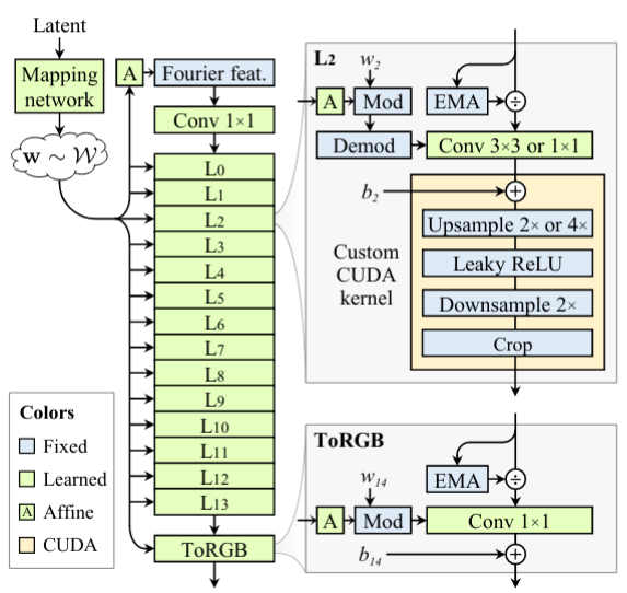Network architecture of the "Alias Free GAN" network.

Mapping Network

The mapping network transforms a normally distributed latent to an intermediate latent code $$w$$. This follows the StyleGAN 2 architecture.

Affine Layer

The authors were motivated to introduce a learned affine layer that outputs global translation and rotation parameters for the input to the Fourier features, because each layer in the network has a limited capability at introducing global transformations, such that to let the orientation vary on a per-image basis the generator should be able to transform input noise $$z_{0}$$ based on $$w$$. Therefore the affine layer outputs translation and rotation parameters used as input to the Fourier features.

Fourier Features

In StyleGAN2 the input model is a learned constant of shape $$4 \cdot 4 \cdot 512$$. In this paper, however, the authors decided to use Fourier features. Defined in [2], Fourier features  involves the Fourier transform of a shift-invariant kernel. The parameters from the affine layer are used as input to the Fourier feature space in this paper.

The key advantage to note here is that since the Fourier features are sampled from a continuous space, the equivariance metrics can be computed exactly without having to approximate the transformation operation in the discrete space. Furthermore, it is suggested that sampling features in this way ensures less of a positional encoding bias.

Experiments

In the paper a large number of ablation experiments are performed; in fact over 92 GPU years of computation was used (it would take 92 years to run all the experiments with 1 GPU). In this section, we will go through some of the different network configurations utilized by the authors to finally end up with the network that produced the videos at the start of the blog and see how the equivariance increases.

In the figure below a summary of all the network configurations is provided, along with FID, EQ-T (equivairant to translation metric) and EQ-R (equivariant to rotation metric).

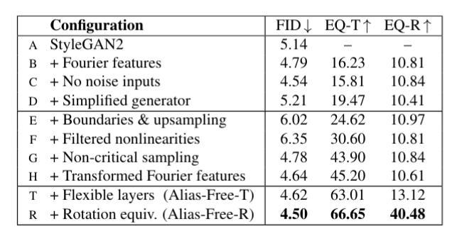Summary of all the various configurations tested. EQ-T and EQ-R is the equivariant translation and equivariant rotation metric.

The notable configurations to discuss is the Alias-Free-T and Alias-Free-R configurations.

Visual differences between the configurations in the table above, in terms of translation and rotation can be seen in the videos below.

T: Flexible Layers

Recall earlier that a low-pass filter is applied after the nonlinearities and the downsampling operations to reduce the introduction of novel frequencies and aliasing. In configuration T, a variable attenuation and cutoff frequency is added for each layer of the network. These values can be seen below. Why does this make sense to do?

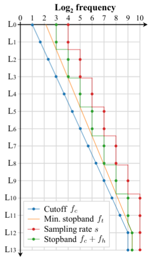The flexible frequency schedule used for each layer of the network.

Well, in low resolution sections of the network the transition band endpoint should be larger, to maximise attenuation in the stopband; ensuring less alias in the low resolution feature maps. In simpler terms, this means that most high frequencies are removed. Whereas in the high resolution feature maps, it should be the opposite, such we are able to match the high-frequency details of the training data. Applying this flexibility along with the non-critical sampling (config G) improved the EQ-T metric greatly. Non-critical sampling essentially just means that frequencies above the Nyquist limit are removed.

R: Rotation equivariance

This final configuration takes everything from above, and adds rotation equivariance. As explained previously, setting all convolution kernels to be of size $$1\;x\;1$$ instead of $$3\;x\;3$$ ensures that rotation equivariance is satisfied. Note however that the number of channels in each layer is doubled. Notwithstanding the number of learnable parameters in the network being 56 % fewer, the FID was unaffected.

An interesting result of improved rotation equivariance is that when generating beach scenes, it appears that camera movement is learnt by the generator:

Relevance to AI-based Compression

Here we speculate on how the advances of this paper may be relevant to us.

1. Equivariant/anti-aliased GANs may have nontrivially-different latent spaces from standard architectures.
   
   The videos of texture sticking in latent exploration shows that StyleGAN 2 (and likely most standard networks) make use of unintended positional encoding. Karras et al. show that their changes give the latent space a noticeably different behaviour.
   
   Furthermore, Karras et al. provide the following visualisation of some selected feature maps:

Clearly Karras et al.'s modifications have lead the model to learn fundamentally different representations in some of its channels.

However, an encoder-decoder pipeline may be very different to their investigation - having a loss that depends on the original and decoded image may mean our networks do not suffer the same problems. This would be easy to check (perturb the input and output by the same transformation and see how this affects the validation loss).

2. At Deep Render, we've seen ringing artifact appear in a few bleeding edge research questions. What's interesting is that ringing is in some sense the inverse of aliasing - too much anti-aliasing causes ringing. Perhaps this paper nudges us towards some signal processing ideas that appear again in future.

Limitations

Here are some limitations of this paper that are worth noting:

• Karras et al. write that it may be a limitation that they only modify the StyleGAN 2 generator - they do not make the discriminator equivariant.
  
  
• The paper makes heavy use of FID scores - most changes are justified through effect on FID score, but we know that this isn't necesarrily the best way to measure visual quality.

Conclusion

The modifications required to obtain an efficient, more equivariant GAN are non-trivial and required years of GPU computations. Nevertheless, the results are fascinating and temporally visually superior to any previous GAN work. For a more in-depth discussion of the implementation required to do this, please see the extensive appendix provided by Karras et. al.

Sources

[1] Matthew Tancik, Pratul P. Srinivasan, Ben Mildenhall, Sara Fridovich-Keil, Nithin Raghavan, Utkarsh Singhal, Ravi Ramamoorthi, Jonathan T. Barron, Ren Ng: “Fourier Features Let Networks Learn High Frequency Functions in Low Dimensional Domains”, 2020; [http://arxiv.org/abs/2006.10739 arXiv:2006.10739].

[2] Ali Rahimi, Ben Recht, "Random Features for Large-Scale Kernel Machines"m [https://people.eecs.berkeley.edu/~brecht/papers/07.rah.rec.nips.pdf]