by Bilal Abbasi and Chris Finlay

tl;dr We outline inter-frame compression techniques in the H.26x family of coding formats. We emphasize the motion compensation and motion prediction modules, with an emphasis on the H.265 (HEVC) format.

Introduction

Traditional video compression achieves remarkable compression rates by exploiting temporal correlations between successive video frames. In this blog post, we will provide a high-level overview of how exactly this is done. We will focus on the H.26x series of video coding formats, and will pay particular attention to H.265 (or HEVC), standardized in 2013.

Motion Compensation

All video compression algorithms (both traditional and AI-based) have used motion compensation in some form or another. The idea is quite simple: suppose you have a series of video frames, and you know the motion vectors which transform each successive frame to the next. Rather than encoding each frame individually, encode instead only the relative difference between each frame.

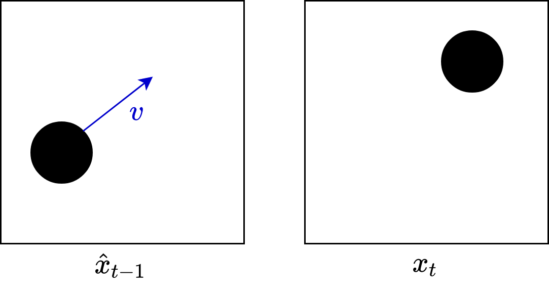
In particular, it is the relative difference between the prior frame warped by the known motion vector, and the current frame, which is encoded. To illustrate: suppose we have a ground-truth frame $$x_t$$ at time $$t$$, and the reconstructed frame $$\hat x_{t-1}$$ at time $$t-1$$. Suppose also we have somehow deduced the motion vector $$v$$ which accounts for (most of) the changes between these two frames. Then, it is the residual difference

$$r_t = x_t - \mathscr F(\hat x_{t-1}, v)$$ ... (1)

between these frames which is actually encoded. Here $$\mathscr F(\cdot\;, v)$$ is the function which transforms an image under a motion vector $$v$$. This is variously called motion compensation (in video compression), a flow (math, physics and elsewhere), and warping (in computer vision). In traditional compression, this residual is chopped into blocks, quantized and encoded via the DCT transform; in AI-based compression the residual is encoded via a neural-network with side-information.

At decode time, the reconstructed frame $$\hat x_t$$ is recovered simply as

$$\hat x_t = \mathscr F(\hat x_{t-1}, v) + \hat r_t$$ ... (2)

where $$\hat r_t$$ is the decoded residual. This process is then repeated for each successive frame.

Why encode the residual rather than each individual frame? Simply because the residuals are typically very sparse, and therefore extremely easy to entropy encode. For example, suppose we have the following example of a moving ball:

We know the previous decoded frame, the motion vector, and the ground-truth current frame. Therefore, we compensate the prior frame using the motion vector, and calculate their difference:

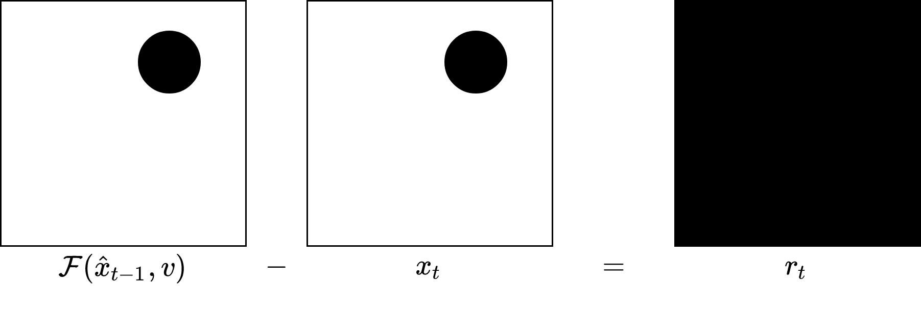
In this contrived example, the difference is all zeros (black), and hence is extremely easy to entropy encode.

Motion compensation in traditional compression

Up until this point, we have assumed that the motion vector is given to us. Of course, this is almost never the case. Instead, we must use some sort of motion estimation algorithm to calculate the motion vectors.

In traditional compression, including the H.26x formats, a block-based approach is used. Each image is cut up into macroblocks of $$N \times N$$ pixels (eg, $$16 \times 16$$ or $$8 \times 8 $$). Then, for each block in the current frame, a search algorithm is used to find the closest matching block in the previous frame. The relative change between the current block and the closest matching block in the previous frame exactly defines the motion vector. The final result of this procedure is illustrated in the following figure. Note that the matched block on the previous frame does not necessarily lie on the fixed macroblock grid.

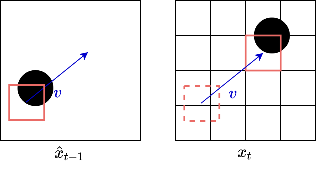
Figure 1. A search is performed over all blocks of the preceding image to determine the best matching prior block. The best matching block determines the motion vector.

There are countless motion estimation algorithms (also known as optical flow estimation), and a discussion of these algorithms is outside the scope of this blog post. Interestingly, the H.26x formats do not specify a motion estimation algorithm; they let each codec implementation choose which motion estimation algorithm to use.

The final result is that each macroblock in the current frame is given a motion vector, which is then used to encode the frame residual (1).

Motion Prediction

However, there is no free lunch. The motion vectors $$v$$ must themselves be encoded and decoded, for how else can the reconstruction $$\hat x_t$$ be recovered from the motion compensated prior frame? Note that at decode, for Equation (2) to be executed, we actually need $$v$$!

In practice, it is too expensive to code the motion vectors themselves. Indeed, naively encoding motion vectors can incur more cost than straight-up encoding standalone images!  So, much like image blocks, we instead code the residuals between the motion vectors and predictions of the motion vectors. These predictions are typically denoted as $$MV$$.  The exact details of how motion vector predictions are generated depend on the video format. However, all prediction methods rely on previously decoded motion vectors, much like block intra predictions in traditional image compression. We will detail per-format specifics in the following sections.

Having calculated the motion predictions, only then can the motion vector residual be computed. The residual between the ground-truth motion vector $$v$$, and the prediction $$MV$$ is known appropriately as the Motion Vector Difference ($$MVD$$):

$$MVD = v - MV$$

The $$MVD$$ is quantized, and sent in the bitstream via a custom entropy encoding module (who's details are rather technical and will not be covered here).

As a side remark, we note that it is the reconstructed motion vector $$\hat v = MV + \widehat{MVD}$$ which is used to actually compute the motion compensation residuals in Equation (1), and for image recovery in Equation (2). We emphasize ground truth motion vector $$v$$ is not used, for it is not available at decode time.

In summary, at decode time, the entire reconstruction process proceeds as follows.

1. $$\widehat{MVD}$$ is recovered from the bitstream
   
   
2. Motion vector predictions $$MV$$ are generated using previously decode information (more on this below)
   
   
3. The reconstructed motion vector is acquired $$\hat v = MV + \widehat{MVD}$$
   
   
4. Motion compensated residuals $$\hat r_t$$ are recovered from the bistream
   
   
5. The actual image is recovered via $$\hat x_t = \mathscr F(\hat x_{t-1}, \hat v) + \hat r_t$$

To illustrate motion prediction in practice, we now turn to two older (simpler and easy-to-understand) formats, H.261 (standardized in 1988!) and H.263 (standardized in 1996).

H.261

H.261 was the first truly practical video compression format.  It uses a uniform macroblock grid structure for each of the channels. The macroblocks in each frame naturally have a correspondence to prior frames, since they remain unchanged.

For motion prediction, H.261 takes the simplest approach. Frames are decoded in their temporal order. H.261 exploits the fact that not only are there strong temporal correlations between frames, but also between motion vectors. Therefore, H.261 defines the motion vector prediction of the current block to simply be the motion vector of the previous block $$MV=\hat v_{t-1}$$. Therefore, $$MVD$$ in this case is just the difference between successive motion vectors of the same macroblock:

   $$MVD_t = v_t - \hat v_{t-1}$$

We emphasize H.261 motion predictions rely on temporal correlations between the motion vectors. Refer to Figure 2.

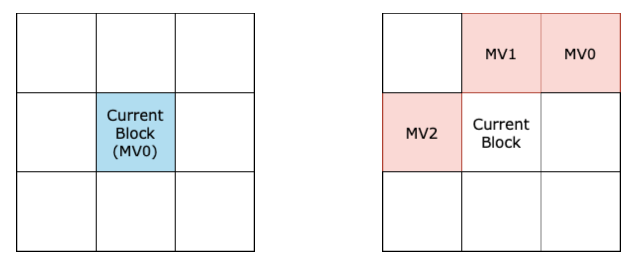Figure 2. Illustration of the blocks (blue for temporal and red for spatial) used for motion vector prediction between different coding methods. For H.261 (left), only the same block in the previous frame (MV0) is considered, whereas for H.263 (right), previously decoded spatially neighbouring blocks (MV0, MV1, MV2) are considered.

H.263

H.263 also uses a uniform macroblock grid structure to partition the input image. One of the key differences, however, between H.261 and H.263 is that H.263 forgoes the use of previous temporal motion vectors, and instead takes advantage of the spatial correlations between neighbouring blocks. This is very similar in spirit to intra-predictions in traditional image codecs. More precisely, with Figure 2 in mind, the $$MV$$ assigned to the current block is given by the component-wise medians of the $$MV$$s of the neighbouring blocks. In other words:

$$MV_x = \text{median}(MV0_x, MV1_x, MV2_x)$$
$$MV_y = \text{median}(MV0_y, MV1_y, MV2_y)$$

In the case where a neighbouring block falls out of the image domain, the motion vector for that block is set to $$(0,0)$$. Using the neighbouring blocks allows for better spatial correlation in the prediction motion vectors, making the resulting motion vector differences easier to encode.

Furthermore, for better accuracy of the flow, H.263 also allows for non-integer directions. That is, the motion-compensated reference macroblock can lie off the pixel-grid (refer to Figure 1). Motion compensation is then achieved via interpolation onto the pixel-grid.

H.265/HEVC

We now turn to H.265, also referred to High Efficient Video Coding (HEVC), standardized in 2013. H.265 has the distinction of being the most recent H.26x format with some adoption (accounting for ~10% of all video streams in 2020 [4]). Though it is not as predominate as its older sibling H.264 (AVC), it is more modern, with good 4k support.

H.265 follows the same development trend as older formats in the H.26x series: it builds on prior existing components, incrementally changing various components of the pipeline. Among the changes introduced, the most significant for inter-frames are: variable macroblock sizes, Advanced Motion Vector Prediction (AVMP), and block merging. Each of these changes will be discussed in this section.

CTU partitioning 

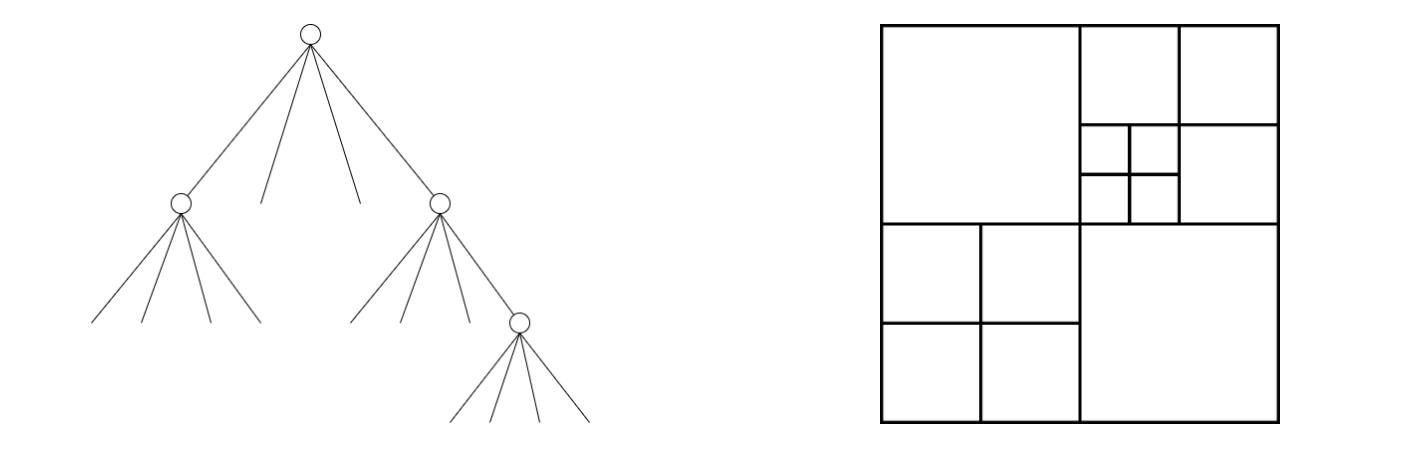
Figure 3. Diagram of quadtree used to partition an image into variable size blocks. Left: Visualization of underlying tree structure. Right: The resulting partition.

One of the major contributions of HEVC is its shift away from a structured grid of macroblocks of a fixed size (as in H.261 and H.263), to an irregularly structured grid of macroblocks of varying sizes.

Each frame is divided into $$64 \times 64$$ blocks, called Coding Tree Units (CTUs). Then, depending on the complexity of the frame,  the frame is recursively broken down into smaller blocks, called Coding Units (CUs). This is done by halving the resolution at each step using a quadtree (refer to Figure 3). The smallest allowable block size is $$4 \times 4$$. The actual decision on whether or not to further partition a particular branch (CU) in a tree is based on optimization of rate and distortion. This results in a semantically meaningful quadtree partition, and much improved rate-distortion curves, but comes at the cost of a higher computational overhead relative to a uniform macroblock grid.

Advanced Motion Vector Prediction

Figure 4. Illustration of block candidates used for motion prediction in HEVC. Red blocks are spatially neighbouring blocks and blue blocks are temporally neighbouring blocks. Note that in this case, the grid of macroblocks is unstructured due to the varying block sizes.

Advanced Motion Vector Prediction (AVMP) is the method used by HEVC to generate motion vector predictions, which are used to compute motion vector differences (as described earlier). AMVP generates MVs by considering candidates of motion vectors at a time, among which a select few will be chosen. For a given block, the candidates are stored in a list as indices. When an appropriate block has been chosen, its index is sent in the bitstream. During decoding, the decoder will generate the same list of candidates and will have access to the index pointing to the block that was chosen by the encoder, thereby knowing exactly which MV to select.

As opposed to H.261 and H.263, block candidates are drawn from both spatially and temporally neighbouring blocks. Referring to Figure 4, spatial candidates $$\{MVa0, MVa1, MVa2, MVb0, MVb1\}$$ are the adjacent blocks found on top and to the left of the current block. Since we cannot look to the right or bottom of the current block (as these will not have been decoded yet), HEVC also considers blocks from the previously decoded frame ($${MVt0, MVt1}$$). Moreover, one of these temporal blocks is a block that is co-located with the current block ($$MVt1$$). The choice of these blocks as candidates was made from extensive ablations.

The number of blocks chosen from the candidates varies, but in general is up to two spatial blocks (one from $$\{MVa0, MVa1, MVa2\}$$ and one from $$\{MVb0, MVb1\}$$) and one temporal block. Among these blocks, a final block is chosen.  The final block is chosen to be the best block minimizing the MVD residual, and this choice is transmitted in the bitstream. However, before transmitting, the MVs are scaled proportional to their temporal distance from the current frame [2]. The temporal distance is computed based on the difference between the temporal index of the current block and the temporal index of the chosen block. The reason this is necessary is because some neighbouring blocks may use an MV from an even earlier frame. To take this into account, HEVC scales the MVs by weighting them according to this distance.

The motion vector difference is computed the same way as in H.261 and H.263, and it is this value which is quantized and encoded.

Merge Mode

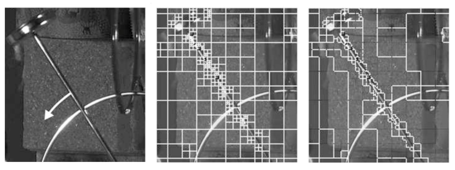
Figure 5. Depiction of excessive refinement from the quadtree partitioning, and the resulting simplification. A frame of a swinging pendulum (left), whose motion is indicated by a white arrow, is partitioned with a quadtree (center). In regions where the same or no motion occurs (along and away from the arm, respectively), there is redundant partitioning. Block merging results in a simplified partition (right), that consolidates redundant information between neighbouring blocks. Source: High Efficiency Video Coding (page 121, Figure 5.6) [2].

The added robustness of having variable sized macroblocks does not come for free. One unfavourable outcome is that the resulting tree may have regions that are too refined. In other words, there may be regions in which neighbouring blocks may share motion information, thereby making it pointless to separate them with a border. Consider Figure 5, for example, in which a frame of a moving pendulum, naively partitioned with a quadtree, may needlessly refine regions that contain no motion (i.e. motion vectors that are $$(0,0)$$). One can eliminate redundancies by merging some blocks together. This does not just apply to adjacent regions that have zero motion; movement along the pendulum arm, for neighbouring blocks, is roughly the same as well.

HEVC addresses the above concern by introducing a block merging module into the pipeline to eliminate and reduce redundancies in coding. Adjacent blocks with identical, or nearly identical, motion vectors are "merged" into one large unit, who all share the same underlying motion vector. This merging procedure has the effect of massively reducing the amount of information needed to encode motion vectors. 

The block merging module is similar to the process used by AVMP. It operates by considering several candidates for block merging at a time. These candidates are identical to those used for AVMP (shown in Figure 4). As in AVMP, only a select few are chosen from the available candidates. In this case, it is up to four of the spatial blocks, and one of the temporal blocks. Blocks are considered in a sequential order, gathering data that is not repeated among other blocks. If the current block's motion vector is very similar to a prior candidate block, the two are merged, and share the same underlying motion vector.

In addition to merging, H.265 has a skip feature, which is a flag to indicate that the motion vector of the current block has not changed from the previous frame. This is particularly important for static regions of the image.

H.266/VVC

Here we briefly remark on motion compensation in the latest of the H.26x formats, standardized in 2020. H.266 builds atop H.265 by considering affine block transformations. All previous H.26x formats performed motion estimation by translating macroblocks -- the translation being given by the motion vector. H.266 extends this concept by allowing for affine transformations of each macroblock. In other words, macroblocks may be translated, resized, rotated, or sheared. This introduces a very heavy computational cost at encode time (the motion estimation algorithm now has a very large search space), and necessitates encoding additional affine information into the bitstream (all details of the affine transform, not just the motion vector, must be encoded). H.266 devotes much effort into overcoming these problems introduced by this added complexity.

Conclusion

In this blog post we outlined two key techniques of traditional video compression, motion compensation and motion prediction. We illustrated these techniques via the H.26x family of compression formats, with an emphasis on H.265. With each successive format, we see an increase in complexity of the motion compensation and motion prediction algorithms.

References

Media

How Video Compression Works

Video Coding Standards - from H.261 to MPEG1,2,4,7 - to H.265 MPEG-H

Literature

[1] Zhang, Yongfei, et al. ‘Recent Advances on HEVC Inter-Frame Coding: From Optimization to Implementation and Beyond’. IEEE Transactions on Circuits and Systems for Video Technology, vol. 30, no. 11, Nov. 2020, pp. 4321–39. DOI.org (Crossref), https://doi.org/10.1109/TCSVT.2019.2954474.

[2] Sze, Vivienne, editor. High Efficiency Video Coding (HEVC): Algorithms and Architectures. Springer, 2014.

[3] Li, Ze-Nian, and Mark S. Drew. Fundamentals of Multimedia. Second edition, Springer, 2014.

Blogs

[4] Traci Ruether, 'Video Codecs and Encoding: Everything You Should Know', 2021. URL https://www.wowza.com/blog/video-codecs-encoding, accessed 2022-03-18.

[5] Denis Fedorov, 'Affine Motion Compensated Prediction in VVC' 2021. URL https://vicuesoft.com/blog/titles/Affine_Motion, accessed 2022-03-18.