-
 ALEX CHERGANSKI 24 Nov
diffusion models
markov chains
probabilistic modelling
variational inference
normalising flows
discrete distributions

a review by Alex Cherganski and Chris Finlay
TL;DR Denoising diffusion models are a new(ish) class of exciting probabilistic models with (a) tractable likelihood estimates, and (b) impressive sampling capabilities. This review focuses on discrete diffusion models, which have yielded impressive results on discrete data [2] (such as modeling quantised images or text).
Introduction
As machine learning practitioners, our day-to-day involves fitting models to unknown data distribution. These models usually are required to do at least one of two things: (1) provide a likelihood estimate (you give me a data sample, my model tells you how likely that data is); and/or (2) generate real-looking data by sampling from the model distribution. These are respectively the tasks of probabilistic inference and generative sampling. Some classes of models can only tractably do one of these two tasks (for example GANs can only generate images). However, in an ideal world, we would love models that can tractably do both.
This has led researchers to develop a host of tractable models capable of both inference and sampling, including for example VAEs, normalizing flows, and autoregressive models (like PixelCNN). In this review, we will study yet another tractable model for both inference and sampling: the denoising diffusion model.
Denoising diffusion models were first brought to the machine learning community in 2015 by Sohl-Dickstein et al. [1] (though the method stems from thermodynamics). However denoising diffusion models went largely unstudied until 2020 when two separate groups (Ho et al. [3] & Song et al. [4]) published impressive results employing the method on image data.
In broad strokes, the idea of denoising diffusion models is simple:
- during generative sampling, noise will be sampled from a simple & tractable known distribution. It will then be progressively cleaned via repeated applications of a learned denoising model. This will be called the reverse process. Importantly, each application of the learned denoising step will be stochastic, and so each denoising step comes with a parametric probabilistic model $$p_\theta (x_\text{clean} | x_\text{noisy})$$.
- during probabilistic inference, a data sample (such as an image) will be progressively corrupted by repeated applications of a known (fixed) corruption process (such as a known and fixed diffusion kernel). Each corruption step is noisy, and so also comes with a fixed probabilistic model $$q(x_\text{noisy} | x_\text{clean})$$. This corruption process iteratively transforms the data distribution to a simple & tractable known distribution. This will be called the forward process. Log-likelihood estimates are given by evaluating the probability under the simple & tractable known distribution. Then, a sum of correction factors is applied to this estimate using the log-ratio between the forward and backward probabilistic models $$\log \frac{p_\theta (x_\text{clean} | x_\text{noisy})}{q(x_\text{noisy} | x_\text{clean})}$$
For students of the more well-known Normalizing Flows, this general setup should seem awfully familiar. For illustration, let's recount their similarities. In both Normalizing flows and Denoising diffusion models, in generation (sampling), noise is transformed by repeated application of some backward process (aka reverse process; aka inverse function). Moreover, in both Normalizing flows and Denoising diffusion models, probabilistic inference is done by transforming data to some simple & tractable distribution by repeated application of a forward process, evaluating the simple distribution, and then correcting this estimate via some change-in-probability factor.
Normalizing flow | Denoising diffusion | |
Probabilistic inference | Evaluate simple distribution; correct via log-determinant of deterministic map's Jacobian | Evaluate simple distribution; correct via log-likelihood ratio between forward and backward stochastic process |
Sample generation | Sample from simple distribution; iteratively apply deterministic backward process | Sample from simple distribution; iteratively apply stochastic backward process |
This similarity is not a coincidence: another way of viewing Denoising diffusion models is as a stochastic Normalizing flows [4] (at least, on continuous data). In the continuous case, really the only major difference is how the correction factor is computed, stemming from the fact one uses stochastic transformations, and the other deterministic. For a further discussion of the relationship between their respective correction factors see [5].
In the continuous setting, Denoising diffusion models have yielded both impressive log-likelihood scores on many standard image datasets, and high-quality image generation [3-4], arguably outperforming Normalizing flows. However, Denoising diffusion models have one very attractive feature that Normalizing flows lack: they are easily defined on discrete data. This will be the main focus of this blog post. We will review the recent paper by Austin et al. [2], which studies Discrete Denoising diffusion models (abbreviated as "D3 models"). In so doing, today we will
- recap Markov processes, a necessary prerequisite;
- define D3 models, via their forward and backward stochastic (Markov) processes;
- explain precisely how to evaluate the log-likelihood of a D3 model (and in so doing, train via minimizing an upper bound on the negative log-likelihood)
Markov chains & processes
The entirety of this blog will deal with modeling discrete data. In other words, each data sample $$x$$ can take on only one of say $$K$$ possibilities, like for instance a finite set of integers $$x \in {[1, 2, \dots, K]}$$.
We can then equate discrete probability mass functions ("distribution") on this space with a vector $$\boldsymbol{q}$$ of length $$K$$, with positive entries that sum to one. Then, we equate the probability $$q(x=i) = \boldsymbol{q}_i$$ with the $$i$$-th entry of the vector.
Probability mass functions so defined are called the Categorical distribution, and you will sometimes see this written as $$q(x) = {Cat}(x; \boldsymbol{q})$$.
D3 models work by transforming these categorical distributions iteratively over a series of time steps $$t=0,\dots,T$$, using a Markov chain. A Markov chain is defined using a transition probability matrix $$\boldsymbol{M}$$, who's entries $$\boldsymbol{M}_{ij}$$ define the probability of transforming state $$x=i$$ into state $$x=j$$.
Now, suppose we are given a distribution $$\boldsymbol{q}^{(t)}$$ (written as a row-vector). At each time step, we update the distribution via
$$\boldsymbol{q}^{(t+1)} = \boldsymbol{q}^{(t)} \boldsymbol{M}$$
The nice thing about this update rule is that it defines a conditional probability model: $$q (x^{(t+1)} | x^{(t)} )$$. If we want to know the probability of a data point $$x^{(t+1)}=i$$ at time step $$t+1$$, all we need to know is the Markov transition matrix, and the probability vector at the previous time step. Nothing else is needed -- this is the so-called Markov property. To reiterate, the probability distribution at time $$t+1$$ only depends on the previous time-step's distribution and the transition matrix, nothing else.
Thus, suppose we are given a whole sequence of states $$x^{(0)}, x^{(1)}, \dots, x^{(N)}$$, and wanted to compute the probability $$q (x^{(N)})$$. Using the Markov property, we progressively expand probability as
$$\boldsymbol{q}^{(N)} = \boldsymbol{q}^{(N-1)} \boldsymbol{M} = \boldsymbol{q}^{(N-2)} \boldsymbol{M}^2 = \dots = \boldsymbol{q}^{(0)} \boldsymbol{M}^N$$
What happens when we send $$N \rightarrow \infty$$? Many Markov chains (but not all) have the property that by repeating this procedure enough times $$\boldsymbol{q}^{(N)}$$ will reach a stationary distribution $$\boldsymbol{\pi}$$. The stationary distribution is a left-eigenvector of $$\boldsymbol{M}$$ with eigenvalue of $$1$$, ie it solves $$\boldsymbol{\pi} = \boldsymbol{\pi} \boldsymbol{M}$$.
Random bit example
Let $$X^{(0)}$$ be a one dimensional Bernoulli random variable (i.e. a random bit with some probability $$p$$ of being "on", and a probability $$1-p$$ of being "off" ). This data is, of course, discrete with two possible states "on" or "off". Let's let $$X^{(0)}$$ represent a data sample at the initial time step. Define a Markov transition matrix
\[
\begin{align}
M =
\begin{bmatrix}
1 - \varepsilon & \varepsilon\\
\varepsilon & 1 - \varepsilon
\end{bmatrix}
\end{align}
\]
where $$\varepsilon$$ is some small number. What this transition matrix says, is if you are in the "on" state, you have a high $$1-\varepsilon$$ probability of staying in the "on" state, and an $$\varepsilon$$ probability of switching to the "off" state. Similarly, if you are in the "off" state, you have a high probability of remaining "off", and a low probability of switching "on".
It is fairly easy to work out that the stationary distribution in this example is $$\boldsymbol{\pi} = [\tfrac{1}{2}, \tfrac{1}{2}]$$.
Chess example
As another example consider a random walk of a king piece in a 8 by 8 chess board. The king moves at each time step with a probability of $$\varepsilon$$ (all cardinal directions are equally likely), and stays at its previous position with a probability of $$1 - \varepsilon$$. The following diagram shows the transition probabilities (on a non-border square).
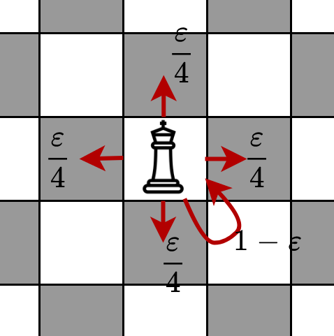 Transition probabilities for the king piece (at a square not on the border)
Let's also assume that the king starts from a fixed square, i.e. all of the probability mass for $$q (x^{(0)} )$$ is on one square.
At each time step, if we observe the distribution $$q (x^{(t)})$$ for large values of $$t$$ we notice that it becomes more and more spread out (i.e. diffused), in exactly the same way that heat diffuses. In other words, the probability mass starts to distribute equally among all the 64 squares of the chess board. In the limiting case $$\lim_{x \to \infty} q ( x^{(t)}) = \tfrac {1}{64}$$ for any value of $$x^{(t)}$$. Thus, in this example, the uniform distribution is the stationary distribution $$\boldsymbol{\pi}$$.
Note that in both of these examples, the Markov transition matrix is a perturbation of the identity. This will turn out to be an important property when later we define our D3 models.
Discrete denoising diffusion models
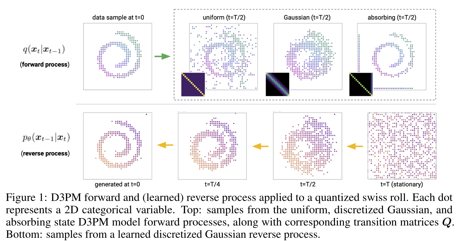
Reproduction of Fig 1 from Austin et al. [2] illustrating the forward process (corrupting the data) and the backward process (denoising the data).
We're now in a position to define Discrete Denoising Diffusion models (D3 models) [1, 2]. D3 models are type of probabilistic model with efficient sampling (generation). Model samples are generated by first sampling data from a simple tractable distribution (aka latent distribution; eg standard multivariate Gaussian or uniform discrete distribution), and then iteratively removing noise using a learned stochastic process. The key here is that the denoising process is learned. How do we learn it? Basically, D3 models are defined to undo some corruption procedure.
To be more precise, suppose we have have a sample $$x^{(0)}$$ drawn from some real-world data distribution, such as an image dataset. The corruption process (called the forward process) will iteratively transform the real-world data by randomly perturbing the data, for example with a fixed diffusion kernel. This will generate a sequence of progressively corrupted data samples $$x^{(0)}, x^{(1)}, \dots, x^{(T)}$$. The denoising model will then iteratively attempt to undo this procedure (i.e. reverse the diffusion, called the reverse process), and tries to create a sequence $$x^{(T)}, x^{(T-1)}, \dots, x^{(0)}$$ reaching back to the initial sample. The forward process corrupts the initial data; the reverse process undoes this corruption.
Forward process
Perhaps unsurprisingly, the forward diffusion process will be a Markov chain
$$q(x^{(t+1)} | x^{(t)}) = \boldsymbol{q}^{(t)} \boldsymbol{M}$$
given some predefined and fixed Markov transition matrix $$\boldsymbol{M}$$. The Markov transition matrix will be defined by the practitioner based on domain specific knowledge. So, for example on 8 bit images, pixels may be perturbed in such a way that colour change probabilities are local, and that drastic colour changes are highly unlikely. Ie, the Markov transition matrix performs perturbations according to some notion of locality (in the Chess example, the king could only jump to neighbouring squares).
If we wanted to, we could define the joint probability of the entire corruption process
$$q(x^{(0)}, x^{(1)}, \dots , x^{(T)}) = q(x^{(0)}) q(x^{(1)} | x^{(0)}) \dots q(x^{(T)} | x^{(T-1)})$$
by applying the chain rule of probability and employing the Markov property. Note that $$q(x^{(0)})$$ is the unknown data distribution we seek to model.
In general, the forward process will use a finite but large number of corruption steps. Crucially, the Markov chain will have a "nice" stationary distribution: the stationary distribution $$\boldsymbol{\pi}$$ should be tractable and easy to sample from. This is because the stationary distribution will be the distribution we sample from in the reverse process. Moreover, we expect that with a large enough number of corruption steps, we expect $$q(x^{(T)}) \approx \boldsymbol{\pi}$$.
Reverse process
So far we have shown how to distort the original data distribution $$q(x^{(0)})$$ into $$\pi (x^{(T)})$$ with iterative addition of tractable noise. The noise here is introduced via a Markov transition matrix. However, the key ingredient of D3 models is a learned reverse process, which attempts to iteratively undo the corruption of the forward process. The reverse process is also defined via a Markov chain
$$p_\theta (x^{(t-1)} | x^{(t)}) = \boldsymbol{p}^{(t)} \boldsymbol{P}_\theta$$
Note that the reverse process is conditioned on forward looking time steps. Here the Markov transition matrix is parameterized somehow, and could actually also depend on the conditioning variable $$x^{(t)}$$. In fact, in most published diffusion models, $$\boldsymbol{P}_\theta$$ is actually a neural network with arguments $$x^{(t)}$$ and $$t$$.
We can also define the joint probability of the entire reverse procedure
$$p_\theta (x^{(0)}, x^{(1)}, \dots , x^{(T)}) = p(x^{(T)}) p_\theta (x^{(T-1)} | x^{(T)})\dots p_\theta (x^{(0)} | x^{(1)})$$
Note that if we were prescient, we wouldn't even need to define & learn a parametric model of the reverse process: we would already know the exact form of the "true" reverse process that undoes the corruption procedure. However, we are not god-like, and so we'll define and learn a parametric reverse process instead, which will be trained to somehow approximate the true (but unknown) reverse process. In general, the model reverse process may not have the same functional form as the true reverse process, however it can be shown that when the random perturbations introduced in the forward process are sufficiently small (the Markov transition matrix is close to the identity), then the backward process has nearly the same functional form as the forward process -- ie the backward process is very close to being a Markov process itself (see [1] for more details). This is why we can get away with defining the model reverse process as a parametric Markov process.
Once the model reverse process is known, we can use it to generate samples from the data distribution $$p (x^{(0)})$$ by first sampling $$x^{(T)} \sim \boldsymbol{\pi} = p (x^{(T)})$$, the iteratively generating the sequence
$$x^{(T)} \rightarrow x^{(T-1)} \rightarrow \dots \rightarrow x^{(0)} $$
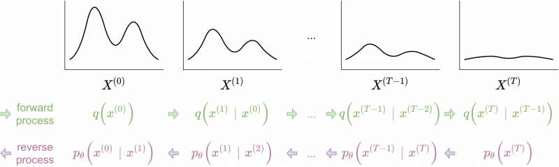 Forward diffusion process and reverse denoising process
What is the probability of the data?
OK, so now we have a way of transforming data $$x^{(0)} \sim q(x^{(0)})$$ to some stationary distribution $$\boldsymbol{\pi}$$, and we have some parametric family of reverse processes that are supposed to be able to turn random noise $$x^{(T)} \sim \boldsymbol{\pi}$$ back into samples from the original data distribution. How do we actually evaluate $$p_\theta (x^{(0)})$$?
Due to the fact that $$p_\theta (x^{(t-1)} | x^{(t)})$$ can be evaluated (we ourselves defined it as a known parametric Markov process), we can evaluate the reverse joint probability $$p_\theta (x^{(0)}, x^{(1)}, \dots, x^{(T)})$$ (just by multiplying out the conditional probabilities -- see the previous section). However, we are interested in calculating the probability of the marginal distribution for our data, ie $$p_\theta (x^{(0)})$$ (we're not so interested in the joint probability of the corruption process, just the probability of the data point):
$$ p_\theta (x^{(0)}) = \sum_{x^{(1 \dots T)}} p_\theta (x^{(0 \dots T)}) $$
That is we will just marginalize out all the later stages of the joint probability of the backward process. Unfortunately, in practice this integral cannot be evaluated tractably. Luckily though there is a nice way to approximate it (and this is one of the big advantages of D3s when compared to other generative models, such as GANs). We will rewrite this marginalization as an expectation over the forward process:
$$
\begin{align}
p(x^{(0)} )
=& \sum_{x^{(1 \dots T)}} p (x^{(0 \dots T)}) \\
=& \sum_{x^{(1 \dots T)}}
\left[
q (x^{(1 \dots T)} | x^{(0)})
\frac {p_\theta (x^{(0 \dots T)})} {q(x^{(1 \dots T)} | x^{(0)})}
\right]
\; \text{(multiply by 1)}\\
=& \mathbb{E}_{x^{(1 \dots T)} \sim q}
\left[ \frac {p_\theta (x^{(0 \dots T)})} {q(x^{(1 \dots T)} | x^{(0)})} \right] \; \text{(rewrite as expectation over forward process)}\\
=& \mathbb{E}_{x^{(1 \dots T)} \sim q} \left[ p(x^{(T)}) \prod_1^T \frac{p_\theta(x^{(t-1)} | x^{(t)})} {q(x^{(t)} | x^{(t-1)})} \right] \; \text{(factor joint probabilities} \\
& \text{via Markov property and chain rule)}
\end{align}
$$
What does this last line say? In order to approximate the probability of a certain data point $$x^{(0)}$$ under the reverse process $$p_\theta(x^{(0)})$$, we need to sample multiple times from the forward process, and then average the expression in the above square brackets. The term inside the expectation is the probability of the end state (we've identified $$p(x^{(T)}) = \boldsymbol{\pi}$$), and a bunch of ratios between the forward and backward conditional probabilities.
How do we train the model?
Training the model comes down to finding the optimal parameters $$\theta$$ that maximise the probability of the data under the reverse model. Assuming our data consists of $$x_1^{(0)}, x_2^{(0)}, \dots, x_N^{(0)}$$ (sampled from $$q(x^{(0)})$$) we want to minimize the KL distance between our model and the true distribution:
$$\min_\theta D_{KL} \left( q(x^{(0)}) \;||\; p_\theta(x^{(0)}) \right)$$
And this can be done by maximizing the log-likelihood of the data
$$
\begin{align}
L =& \max_\theta \mathbb{E}_{x^{(0)} \sim q} \left[ \log p_\theta (x^{(0)}) \right] \\
=& \max_\theta \mathbb{E}_{x^{(0)} \sim q} \left[ \log \mathbb{E}_{x^{(1 \dots T)} \sim q(\cdot | x^{(0)})} \left[ \frac{p(x^{(0 \dots T)})} {q(x^{(1 \dots T)} | x^{(0)})} \right]\right]
\end{align}
$$
The outer expectation will be done by sampling available training data $$x^{(0)} \sim q (x^{(0)})$$. The inner probability $$p (x^{(0)})$$ is approximated by sampling corruption sequences from the forward process $$q (x^{(1 \dots T)} | x^{(0)} )$$.
We can combine both expectations by deriving the variational lower bound with the application of Jensen's inequality:
$$
\begin{align}
L \ge& \max_\theta \mathbb{E}_{x^{(0 \dots T)} \sim q}
\left[
\log \frac{p_\theta\left(x^{(0 \dots T)}\right)} {q\left(x^{(1 \dots T)} | x^{(0)}\right)}
\right] \\
=& \max_\theta \mathbb{E}_{x^{(0 \dots T)} \sim q}
\left[
\log p (x^{(T)})
\prod_1^T \frac{p_\theta\left(x^{(t-1)} | x^{(t)}\right)} {q\left(x^{(t)} | x^{(t-1)}\right)}
\right] \\
=&\max_\theta \mathbb{E}_{x^{(0 \dots T)} \sim q}
\left[ \underbrace{
\log p(x^{(T)}) +
\sum_1^T \log \left\{\frac{p_\theta\left(x^{(t-1)} | x^{(t)}\right)} {q\left(x^{(t)} | x^{(t-1)}\right)}\right\}
}_{\text{having closed form depending on } \theta} \right]
\end{align}
$$
Now we can optimize the above lower bound of the log-likelihood with SGD by sampling from the forward process and evaluating the log probabilities in the square brackets, for which we have closed forms.
We remark that this lower bound has a very similar structure to log-likelihood estimates arising in Normalizing flows:
- $$\log p(x^{(T)})$$ is analytic and easily evaluated, since it is identified with the stationary distribution $$\boldsymbol{\pi}$$. This is an "initial estimate" of the log-likelihood.
- $$\sum_1^T \log \left\{ \frac{p_\theta\left(x^{(t-1)} | x^{(t)}\right)} {q\left(x^{(t)} | x^{(t-1)}\right)}\right\}$$ is a sum of correction terms to the tractable initial estimate.
- Interestingly, when the data is continuous, in the case that the forward process and backward process are deterministic (and so optimally are inverses of each other), the log-ratio terms simplify to log-determinants of the Jacobian, as in Normalizing flows [5]
Discussion of Austin et al.
The recent paper by Austin et al. [2] studies D3 models in great detail, amassing a trove of impressive experimental results on discrete data. Much of the paper is dedicated to architectural design choice.
Much work is needed to properly design sensible corruption processes on the forward Markov chain. For instance, on image data, reflecting or absorbing boundary conditions can be incorporated, and the Markov transition matrix can be defined to have some local structure, such as being discrete approximations of the Gaussian. On text data, Austin et al. employ specialized Markov processes particularly adapted to textual data. The choice of transition matrix is critical for achieving well-performing D3 models. For instance, previous authors had used uniform transition matrices, with poor results. Austin et al. have showed that by choosing Markov transition matrices particularly adapted to the topological structure of the data, far superior results can be obtained over naive choices of the Markov transition matrix.
Many authors [1-4] have found that training is improved when the forward process includes a variable noise schedule, such that the Markov transition matrix $$\boldsymbol{M}_t$$ depends on $$t$$, and moves further from the identity as $$t$$ increases. In the discretized Gaussian case, Austin et al. do this by increasing the variance of the Gaussian proportional to $$t$$.
Despite being discrete models, on image data the results presented in Austin et al. achieve similar sample quality to other (continuous) diffusion models on simple image datasets, but with better log-likelihood scores.
Austin et al.'s results are not competitive with current state-of-the-art models, such as massive Transformer models on text; or the latest and greatest continuous-time continuous state diffusion models [6] in the image domain. However, what this paper does show is that with proper design choices, discrete models can be very competitive with other continuous models.
Many datasets are discrete, but for ease of modeling oftentimes these datasets are embedded in a continuous space, and then modeled continuously. However this can lead to tricky modeling questions, such as "de-quantization" roadblocks, strange gradient issues, and difficulties interpreting log-likelihood measures. By actually modeling discrete data discretely, all these issues are avoided. It is for this reason we are excited about this paper: it shows that diffusion models, with proper design choices, can be very competitive on discrete datasets. We believe with further refinement, D3 models will gain in prominence on discrete datasets.
References
[1] Sohl-Dickstein, Jascha, Eric Weiss, Niru Maheswaranathan, and Surya Ganguli. "Deep Unsupervised Learning using Nonequilibrium Thermodynamics." In International Conference on Machine Learning, pp. 2256-2265. PMLR, 2015. [arXiv] [PMLR]
[2] Austin, Jacob, Daniel Johnson, Jonathan Ho, Danny Tarlow, and Rianne van den Berg. "Structured Denoising Diffusion Models in Discrete State-Spaces." arXiv preprint arXiv:2107.03006 (2021). [arXiv]
[3] Ho, Jonathan, Ajay Jain, and Pieter Abbeel. "Denoising diffusion probabilistic models." arXiv preprint arXiv:2006.11239 (2020). [arXiv] [NeurIPS]
[4] Song, Yang, Jascha Sohl-Dickstein, Diederik P. Kingma, Abhishek Kumar, Stefano Ermon, and Ben Poole. "Score-based generative modeling through stochastic differential equations." arXiv preprint arXiv:2011.13456 (2020). [arXiv] [ICLR]
[5] Nielsen, Didrik, Priyank Jaini, Emiel Hoogeboom, Ole Winther, and Max Welling. "Survae flows: Surjections to bridge the gap between vaes and flows." Advances in Neural Information Processing Systems 33 (2020). [arXiv] [NeurIPS]
[6] Kingma, Diederik P., Tim Salimans, Ben Poole, and Jonathan Ho. "Variational Diffusion Models." arXiv preprint arXiv:2107.00630 (2021). [arXiv]
RELATED BLOGS
 ALEXANDER LYTCHIER
- 18 Nov
 HAMZA ALAWIYE
- 11 Oct
 AARON DEES
- 14 Apr