Abstract

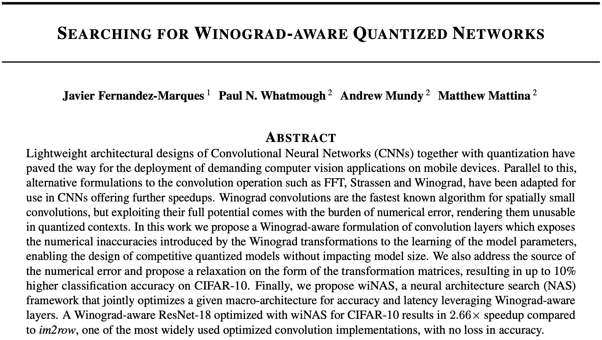
Saif Haq and Jan Xu have chosen to present the paper Searching for Winograd-aware Quantized Networks from researchers at University of Oxford and Arm ML Research Lab. They start the paper review by taking a look at the abstract as a whole, and breaking it down into parts:

Let's divide this into separate parts and elaborate on each of them.

Lightweight architectural designs of Convolutional Neural Networks (CNNs) together with quantization have paved the way for the deployment of demanding computer vision applications on mobile devices. Parallel to this, alternative formulations to the convolution operation such as FFT, Strassen and Winograd, have been adapted for use in CNNs offering further speedups.

Running CNNs on mobile and IoT devices with constrained hardware has necessitated the push for architectural designs with low memory, compute and energy budgets, that can yield fast inference times without overly compromising on the model performance. To achieve this, we can either

(a) adopt lightweight CNN architectures such as smaller kernels, depth-wise or separable convolutions;
(b) quantise our model to lower bit widths;
(c) use alternative convolution algorithms, such as FFT, Strassen and Winograd convolution, instead of direct convolution.

Winograd convolutions are the fastest known algorithm for spatially small convolutions, but exploiting their full potential comes with the burden of numerical error, rendering them unusable in quantized contexts.

In the case of (c), the Winograd convolution is fastest for convolutions with small kernels, often 3x3. In broad terms, it consists of transforming the input and kernel into a Winograd domain, applying the convolution by an element-wise product, and transforming the output back to the original domain. However, certain Winograd algorithms suffers inherently from numerical errors that get exacerbated in quantised models, implying that (b) and (c) are, to a certain extent, irreconcilable.

In this work we propose a Winograd-aware formulation of convolution layers which exposes the numerical inaccuracies introduced by the Winograd transformations to the learning of the model parameters, enabling the design of competitive quantized models without impacting model size.

This paper proposes a way to resolve this incompatibility by introduces Winograd-aware convolutions. This allows the model parameters to account for the numerical errors of Winograd, even in lower-bit networks.

We also address the source of the numerical error and propose a relaxation on the form of the transformation matrices, resulting in up to 10% higher classification accuracy on CIFAR-10.

The paper also proposes a relaxation technique on the Winograd transforms, which further closes the accuracy gap (by up to 10%) between the slow but precise direct convolution and the fast but imprecise Winograd convolution.

Finally, we propose wiNAS, a neural architecture search (NAS) framework that jointly optimizes a given macro-architecture for accuracy and latency leveraging Winograd-aware layers. A Winograd-aware ResNet-18 optimized with wiNAS for CIFAR-10 results in 2.66× speedup compared to im2row, one of the most widely used optimized convolution implementations, with no loss in accuracy.

Lastly, this paper offers a NAS framework that can trade off between accuracy and latency by searching for the best convolution method and bit width in each layer. As we shall soon see, they perform their experiments on actual CPU hardware and notice an impressive speedup compared to direct convolution on classification tasks, with near zero loss in accuracy.

Introduction

In many ML applications, convolutional operations have become a staple. Importantly for us, they are an integral part to our compression pipeline, so finding a small increase in efficiency would bring about large benefits and savings in time and efficient use of compute. As we are trying to port our models to mobile devices, runtime is going to be a big concern in inference. First, we give a general introduction about runtime concepts, before delving deeper into standard Winograd convolutions. These concepts will set the foundations for the paper under question.

So what does it mean to improve runtime? Figure 1 below shows a hierarchy of what can be changed to improve runtime. 

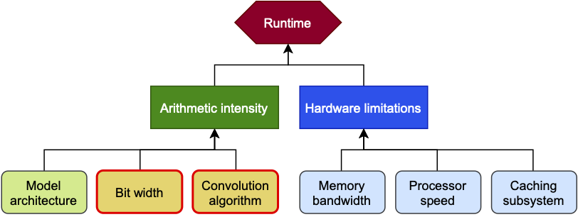Figure 1: A hierarchy of constituents that have an impact on runtime. This blog article focuses on bit width and the convolution algorithm to improve arithmetic intensity, and in turn runtime.

From a high-level overview, the runtime is governed by arithmetic intensity and hardware. The arithmetic (or operational) intensity $$I$$ of an algorithm is the ratio of FLOPS (or performance) and data movement required by the algorithm, measured in FLOPS/byte. The roofline model defines the attainable performance of our algorithm as $$P = \begin{cases} {\large\pi} \\ {\beta} \times I \end{cases}$$ where $$\large\pi$$ is the peak performance and $$\beta$$ is the peak memory bandwidth of the hardware. In other words, if our $$I < \frac {\large\pi} {\beta}$$, the algorithm is memory-bound. If $$I > \frac{\large\pi} {\beta}$$, it is compute-bound. The ratio $$ \frac {\large\pi} {\beta}$$ is sometimes also referred to as compute-to-memory ratio (CMR).

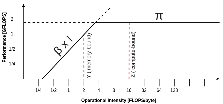Figure 2: The roofline model showing performance estimates of a given compute kernel by showing limitations in either its FLOPS or its data movement.  

Learned image and video decoders generally fall under the category of memory-bound algorithms, due to the large memory transfer between the cache memory / RAM and the ALU of the feature maps and kernels. Therefore, reducing the number of FLOPS would not improve inference speed. This can be seen in the roofline diagram above at $$Y$$, where an excess of FLOPs is being limited by the data movement.

This paper under review focuses on increasing arithmetic intensity by lowering the required data movement. The authors focus on achieving this by varying the convolution algorithm and the bit width rather than model architecture, as shown in Figure 1. This formula below gives some intuition on how data movement can be improved:

$$DM ≈ \text{bit width} \times \underbrace{C \times H \times W}_\text{Model architecture}  \times \underbrace{\frac{(m + r - 1)^2} {m^2}}_\text{Convolution algorithm}  \times \text{caching factor}$$

$$r$$ is the kernel size and $$m$$ is the output tile size of the Winograd convolution (more on this in the next section). The caching factor can be ignored for now. So, to improve data movement, and therefore runtime, we discuss how we could either quantise our model to lower bit widths; or use a faster convolution algorithm that would allow you to perform more operations with the same memory transfer.

Using lower-precision (quantised) networks results in smaller model sizes, faster inference, lower energy consumption, and smaller chip area, which has a direct impact on the data movement [1]. For these reasons, 8-bit arithmetic encoding has been widely adopted in compute-constrained devices.

There are a few ways of performing convolutions. Winograd-based convolutions have quickly gained traction as a preferred approach to implement convolutional neural networks (ConvNet) for small kernels on various hardware platforms because it requires fewer floating-point operations and data movement than standard/direct convolutions (GEMM, normally using the operations im2row and im2col). 

Although Winograd-based convolutions sound great, they do suffer from exponentially increasing numerical errors which increase with the tile size parameter $$m$$. The reason this happens is beyond the scope of this article but if you’re interested, see [9]. Despite the fact that neural networks are known to be to be fairly robust to weight quantisation, this is not the case for when Winograd is used as the numerical inaccuracies get exacerbated with lower bit widths (see Table 2 two sections below).

The Winograd-aware Quantized Network discussed later in the blog post poses a solution that allows the quantised network to accommodate for the numerical errors through backpropagation, allowing learnable parameters to absorb some of this inaccuracy.

Background: Winograd convolution

Before we start presenting the paper, this section provides a quick overview in how the Winograd algorithm works. Principally, Winograd works on the basis of algorithmic strength reduction: swapping out expensive operations such as multiplications with cheaper operations such as additions.

Standard GEMM based convolutions have a lot of overlap in pixels when a filter is convolved over the input. Figure 3 below shows a standard 3x3 convolution being applied to the top left of an image (the 4x4 input). The centre four pixels are used in all four of the matrix multiplications, so this is where Winograd improves on redundant operations.

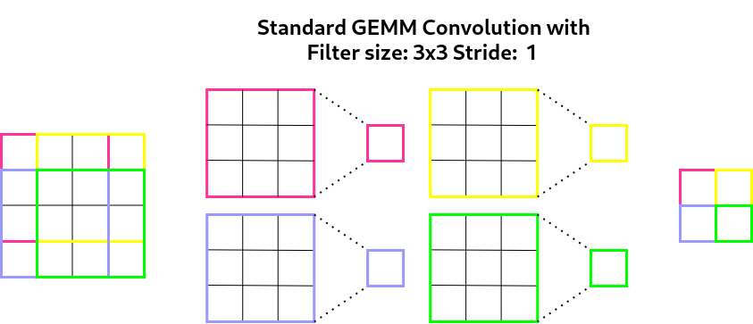Figure 3: A visualisation of the matrix multiplications required to achieve a convolution reducing a 4x4 input to a 2x2 output with a 3x3 filter, using the GEMM (im2col) algorithm.

Instead of having 36 multiplication operations (4 times 3x3) in the example above, a Winograd convolution would instead reduce this to 16 (1 times 4x4); which is a 2.25 increase of algorithmic efficiency for convolutions with filter sizes of 3x3. The Winograd algorithm achieves this by breaking up the input image into overlapping tiles of size $$m + r - 1$$ and performing the convolution in the ‘Winograd domain’, where the convolution is simply a Hadamard product or element-wise multiplication. The Winograd algorithm of input tile $$X$$, weight kernel $$W$$ and output $$Q$$ can be described with the following formula:

$$Y = \underbrace{\mathbf{A}^T\left[ \underbrace{\mathbf{G} W \mathbf{G}^T}_\text{Kernel transform} \underbrace{\odot}_\text{Hadamard product} \underbrace {\mathbf{B}^T X \mathbf{B}}_\text{Input transform}\right] \mathbf{A}}_\text{Output transform}$$

Here, we can see that three transformations need to occur: (i) the input transform using the matrix $$\mathbf{B}^T$$ which transforms the input tile $$X$$ into Winograd space; (ii) the kernel transform using the matrix $$\mathbf{G}$$, which transforms the weight kernel $$W$$ into Winograd space (can be pre-computed so will not affect runtime); (iii) the output transform using the matrix $$\mathbf{A}^T$$, which transforms the output back into the original space. $$\mathbf{B}^T$$, $$\mathbf{G}$$ and $$\mathbf{A}^T$$ are collectively known as the Winograd transformation matrices. A visualisation of this procedure is shown in Figure 4.

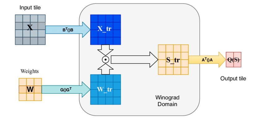Figure 4: $$F(2 \times 2, 3 \times 3)$$ or F2 Winograd pipeline where the input tile and weight kernel have the $$\mathbf{B}^T$$ and $$\mathbf{G}$$ matrices applied respectively, transforming them to the Winograd domain. Then, they are multiplied element-wise (Hadamard product), and the output is finally transformed back to the image domain using the $$\mathbf{A}^T$$ transformation matrix.

The Winograd algorithm can be defined for multiple output tile sizes $$m$$ and kernel sizes $$r$$. The algorithm itself, for a 2D convolution, can be denoted as $$F(m \times m, r \times r)$$. In this paper, the authors focus mainly on 3x3 kernels and refer to $$F(2 \times 2, 3 \times 3)$$ as F2, $$F(4 \times 4, 3 \times 3)$$ as F4 etc.

Each size configuration of Winograd has differently initialised transformation matrices. Most commonly, they are initialised with the Chinese Remainder Theorem or the Cook-Toom algorithm, which requires choosing a set of so-called polynomial points. The choice of these are not trivial, but for small Winograd kernels and output tile sizes, such as F2 and F4, there is a common consensus on the "best" points [4].

The efficiency of Winograd-based algorithms depend directly on the output tile size. Table 1 shows how many input-and-kernel multiplications are required to achieve a convolution at different output tile sizes, assuming a kernel size of 3x3. It is very clear that larger output tile sizes of Winograd enjoy a greater arithmetic complexity reduction factor compared to GEMM convolutions.

However, the numerical imprecision is also closely associated with the output tile size, as well as the bit width of the operation.  The implications of reducing bit width and/or increasing output tile size can be seen from Table 2 below. Next section will explain further the numerical errors encountered when performing model quantisation in larger-tile Winograds.

Numerical errors of Winograd

As previous sections explain, the Winograd convolution inherently suffers from numerical inaccuracies induced by the complexity of the convolution method (F2 vs F4 vs F6) and the bit width of the operation (32-bit vs 16-bit vs 8-bit). This incongruity is shown in the Table 2.

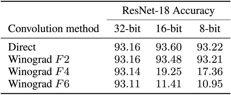Table 2: CIFAR-10 accuracies for a ResNet-18 architecture pre-trained in full precision (float32) with different Winograd convolution methods and bit widths switched on. 

Upon model quantisation, the CIFAR-10 accuracy drops by around 75% with F4 convolutions and over 80% with F6! Whilst F2 still works well in quantised networks, it's clear from this table that quantising a pre-trained model renders Winograd F4 and F6 virtually unworkable. In other words, we can't reap the runtime benefits of both reduced precision arithmetic and the more efficient F4 or F6 Winograds simultaneously; in its current form, we have to choose either or.

Luckily, this paper attempts to resolve this incompatibility and offers a solution for closing this accuracy gap, whilst retaining the speedup from the Winograd algorithm. They achieve this by formulating so-called Winograd-aware networks.

Winograd-aware networks

The core idea is extremely simple, yet effective: during training, instead of direct convolution, every convolution $$z = f(d, g)$$ (slightly different notation from above, but $$z = Y = \text{output tile}$$, $$d = X = \text{input tile}$$ and $$g = W = \text{weight kernel}$$) is explicitly implemented as a Winograd convolution formulated by the equation:

$$z = \mathbf{A}^T [\mathbf{G} g \mathbf{G}^T \odot \mathbf{B}^T d \mathbf{B}] \mathbf{A}$$

This exposes the Winograd transformation matrices to the model training, since the Winograd convolution consists of only backpropable (matrix-matrix multiplication and element-wise multiplication) operations. This means that

• the model weights are exposed to the numerical errors introduced by Winograd so they can account for them;
  
  
• instead of the transformation matrices $$\mathbf{B}^T$$, $$\mathbf{G}$$ and $$\mathbf{A}^T$$ being static (which they normally are), these can be learnable parameters in the layer. This relaxation of the Winograd transforms offers additional flexibility for Winograd-aware layers to adapt around numerical errors, which leads to further narrowing of the accuracy gap introduced in quantised networks.

In the following sections of the paper, the models that include just the first bullet point are termed Winograd-aware, and refer to these models in the experimental results below simply as F2, F4 and so on (with static Winograd transforms). The authors use the suffix '-flex' to denote if the Winograd-aware model also includes the second bullet point, i.e. enables the transformation matrices $$\mathbf{B}^T$$, $$\mathbf{G}$$ and $$\mathbf{A}^T$$ to be learnable.

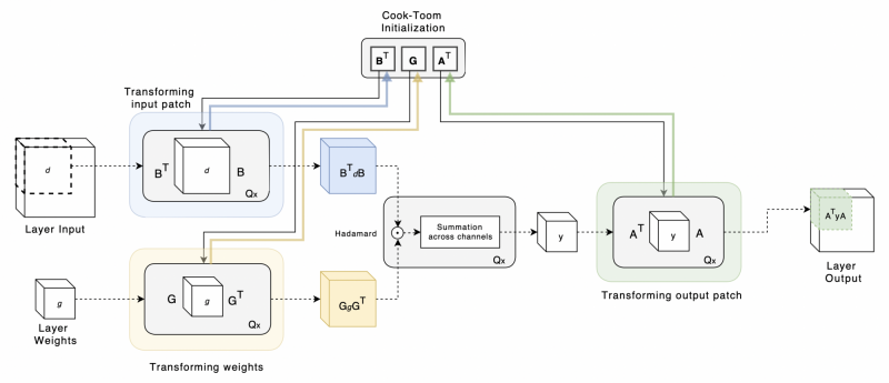Figure 5: The forward pass of a Winograd-aware layer, in which the transformation matrices $$\mathbf{B}^T$$, $$\mathbf{G}$$ and $$\mathbf{A}^T$$ are initialised via Cook-Toom algorithm [4]. If the transformation matrices are part of the learnable set of model parameters, the gradients carried from the loss function would update these (given by the coloured arrows). $$Qx$$ denotes the intermediate quantisation operation that takes place in each step of the algorithm to the desired bit width.

Using Winograd-aware training, how much of the lost accuracy due to model quantisation can we recover when using F4 or F6? The authors studied this by training ResNet-18 architectures [6] on a CIFAR-10 classification task from scratch, comparing configurations for different convolution algorithms (F2, F4 and F6 plus their '-flex' counterpart) and bit widths (32-bit, 16-bit, 10-bit and 8-bit). They also varied the model size with a uniform multiplier for the channel width of the layers (with a width multiplier of 1.0 corresponding to the full ResNet-18). The results can be seen in Figure 6 below.

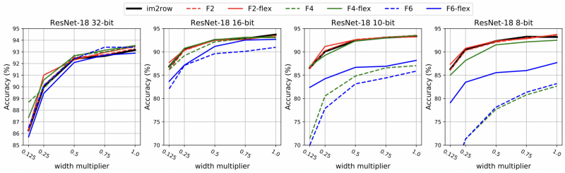Figure 6: Performances of Winograd-aware ResNet-18 architectures on CIFAR-10 for various Winograd algorithms (versus direct convolution or im2row) and various bit widths. In quantised networks, the '-flex' configurations (i.e. those that learn the Winograd transforms) are essential for maintaining high accuracy of the model. 

Firstly, let's compare the Winograd-aware models (static transforms only for now) with the aforementioned accuracy gaps, and focus on width multiplier = 1.0 only. Using F4 convolutions, Winograd-aware training practically closes the gap entirely in 16-bit(!), whilst in 8-bit around 65% of the accuracy is recovered. Using F6 convolutions, almost 80% and 72% of the accuracy is recovered in 16-bit and 8-bit, respectively. In summary, we can narrow the gap significantly by training with Winograd-aware layers, but it is still evident that larger-tile Winograds (F6) struggle more to close the gap when compared to F2 and F4.

Secondly, it's apparent that learning the Winograd transforms is super important for retaining performance in quantised networks, even more so than just exposing the model weights to the Winograd inaccuracies. In the 8-bit experiment, the '-flex' configurations result in 10% and 5% higher accuracies for F4 and F6, respectively, than their non-flex counterpart. This means for F4, the accuracy gap is pretty much closed in 8-bit. Unsurprisingly, there seems to be no discernible difference between F2 and F2-flex at any bit width.

Thirdly, the authors also performed a similar experiment on an 8-bit version of the LeNet-5 architecture [7], which uses 5x5 kernels, on classifying MNIST digits. We won't include the figure here (Figure 5 in the paper), but it basically shows that the '-flex' configuration is again vital in order to use F4 and F6 in such low bit widths.

Lastly, the authors demonstrate that it is possible to take a fully trained ResNet-18 model with direct convolutions (no numerical errors) of a given bit width, and retrain it with F4 convolutions. If Winograd transformation matrices are allowed to evolve during training, it can fully recover the accuracy of the original model within 20 epochs. Figure 7 demonstrates exactly this for an 8-bit model. Note that the pre-training and retraining has to occur in the same bit width; for instance, retraining a 32-bit model in 8-bit would not work.

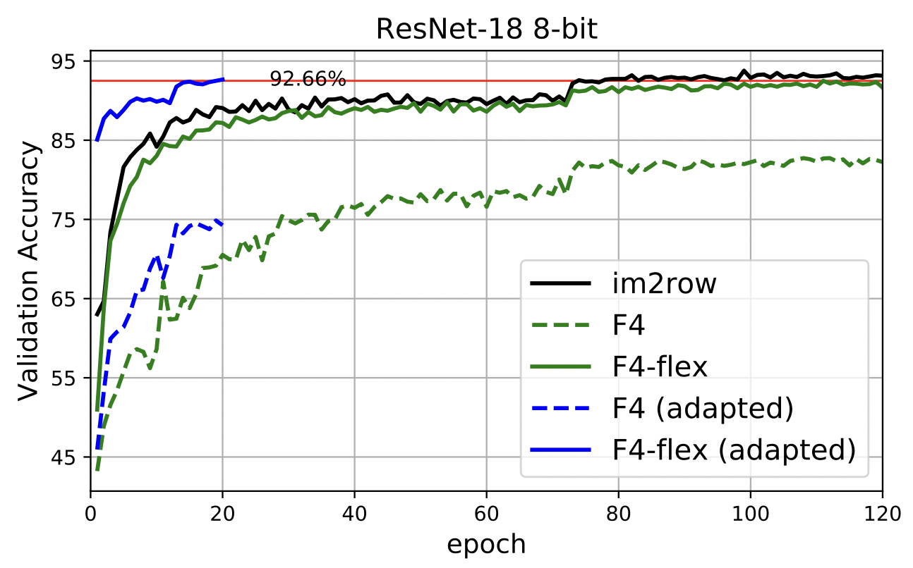Figure 7: Retraining (or adapting) a pre-trained model with im2row convolution (solid black) can be successfully and quickly done for a F4-flex configuration (solid blue), even more so than training the F4-flex model from scratch (solid green). With static Winograd transforms, neither retraining nor training from scratch in F4 yielded good performance. 

One caveat with Winograd-aware training is that it requires very high memory usage, which consequently might slow down training. This is due to the exposure of the Winograd transforms, each of which has intermediate outputs due to the matrix-matrix multiplication that are required for backpropagation. The authors relied on gradient checkpointing [8] to train these models, however may be cumbersome to do for production code.

Therefore, the last mentioned observation is important. One would be able to take pre-trained, quantised models (often having used direct convolution in training) and simply finetune them with a F4-flex configuration, for example. This means you can do the bulk of the training efficiently with direct convolutions, and then apply a short post-training Winograd-awareness scheme before deploying them on mobile chips with Winograd algorithms, whilst expecting only marginal (if any) loss in performance.

wiNAS: jointly optimising for accuracy and latency

Heuristically, larger tile sizes of the Winograd convolution result in lower latencies but lower model performance (or accuracy) due to numerical errors. As we've seen how the accuracy of quantised models can be partially or even fully recovered by employing Winograd-aware layers, let's talk about how to find a good tradeoff between maximising accuracy and minimising latency.

The authors thus present a second contribution in this paper, titled wiNAS, which is a NAS-based framework that "automatically transforms an existing architecture into a Winograd-aware version" that jointly optimises for network accuracy and latency. The NAS operates on a micro-architecture level, with candidate operations (or the operation set) such as different convolution algorithms (im2row, F2, F4 etc.) and bit precisions (float32, float16, int8) per layer.

The authors use a variation of the ProxylessNAS [5], which samples the path stochastically during the search using the architecture parameters $$({a_0, a_1, ..., a_n})$$. These are softmaxed, yielding probabilities $${(p^0, p^1, ..., p^n)}$$, from which the path is sampled. (In actuality, two paths are being sampled in order for gradients to pass through multiple operations.) Similar to ProxylessNAS, the wiNAS formulates the search as a two-stage update process:

1.     Update of model parameters (convolutions, activations etc.) through the loss metric $$\mathcal{L}_{model}$$.

2.     Update of architecture parameters $${a_0, a_1, ..., a_n}$$, where the loss introduces the latency metrics

$$\mathcal{L}_{arch} = \mathcal{L}_{model} + \lambda_1 ||a||_2^2 + \lambda_2 E[\text{latency}]$$

The $$||a||_2^2$$ is a weight decay term on the architecture parameters and the expected latency of a layer $$l$$ is the weighted sum of individual operation latency estimates $$F(o_j^{[l]})$$ for each operation $$o_j^{[l]}$$:

$$E[\text{latency}^{[l]}] = \sum_j p_j F(o_j^{[l]}) = \sum_j \frac {\exp(a_j)}{\sum_j \exp(a_j)} F(o_j^{[l]})$$

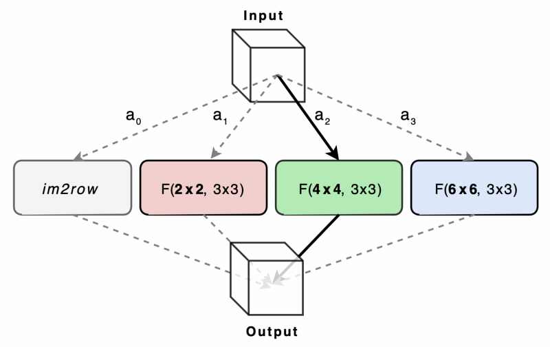Figure 8: The micro-architecture NAS problem formulated by wiNAS for each convolution layer. Here, bit widths is not shown but may also be a second axis to perform search over. 

The $$F(o_j^{[l]})$$ term is precomputed, either analytically or empirically, which is a function of the feature size of $$o_j^{[l]}$$ and quantisation level. The authors chose to compute it empirically on two different ARM Cortex-A CPU cores: A73 and A53 (these will be expanded on in the next section). For each convolution method (im2row, F2, F4 and F6), the operation latency was measured for various feature resolutions and channel sizes, and stored to be used in the NAS training. As such, this joint optimisation framework takes into account both performance losses of the model and the latency of the operations, whose trade-off is controlled by the $$\lambda_2$$ factor in the loss function.

The authors differentiate between two variations of the wiNAS framework:

• $$\text{wiNAS}_\text{WA}$$: the bit width is fixed for all layers, and the search is only over the operation set of convolution algorithms for each layer (im2row, F2, F4, F6)
  
  
• $$\text{wiNAS}_\text{WA-Q}$$: in addition to searching over the operation set of convolution algorithms, it also searches over the operation set of bit widths for each layer (32-bit or FP32, 16-bit or INT16, 8-bit or INT8).

The search for the optimal configuration was performed for 100 epochs on CIFAR-10 and CIFAR-100 on a ResNet-18 backbone. Once completed, the resulting architectures was trained end-to-end as the other Winograd-aware networks. The resulting architectures can be seen in Figure 9.

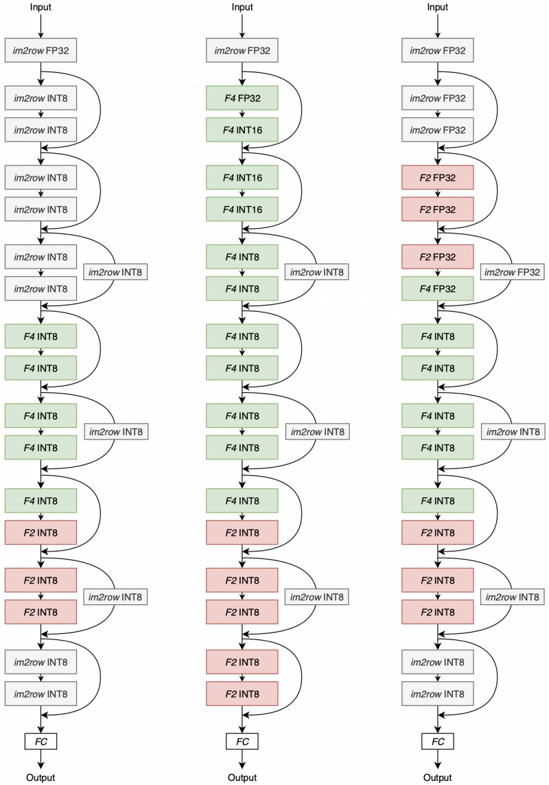 Figure 9: Resulting wiNAS architectures on ResNet-18. 
Left: $$\text{wiNAS}_\text{WA}$$ search, fixed 8-bit width, optimised over CIFAR-100.
Centre: $$\text{wiNAS}_\text{WA-Q}$$ search, optimised over CIFAR-10.
Right: $$\text{wiNAS}_\text{WA-Q}$$ search, optimised over CIFAR-100. 

A discussion on their quantitative performance will be deferred to the next section which is, frankly, the more important takeaway from the wiNAS framework. For now, given this figure, we can do a quick qualitative interpretation:

• The $$\text{wiNAS}_\text{WA-Q}$$ searches prefer larger bit widths in the earlier layers in general.
  
  
• Since CIFAR-100 is a considerably harder classification task than CIFAR-10, those models require higher accuracy in the earlier layers. The $$\text{wiNAS}_\text{WA}$$ search (left) does so with im2row convolutions, whereas the $$\text{wiNAS}_\text{WA-Q}$$ search (right) does so with 32-bit convolutions.
  
  
• Downscaling skip connections seem highly important to maintain good accuracy, since they all were assigned with im2row convolutions.
  
  
• F6 is not selected anywhere; although it could be due to bad luck, it's likely to be due to detrimental effects to model accuracy.

Benchmarking Winograd on mobile CPUs

It is evident that model accuracy or performance stays mostly consistent across various experimental frameworks and hardware types. On the contrary, runtime or latency is extremely hardware-dependent. For that, it's very important to consider the application and the computational resources available for the relevant neural network.

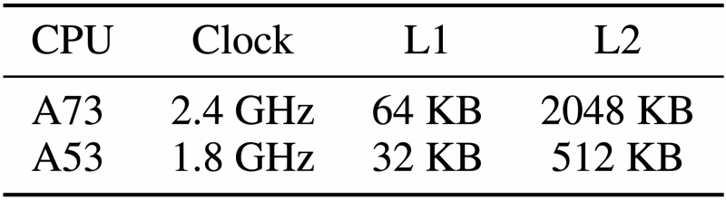Table 3: Key hardware specifications for the two mobile chips tested in this paper. 

In the case of this paper, the authors target the usage of neural networks in chips commonly found in today's off-the-shelf mobile hardware. To this end, they opted for one ARM Cortex-A73 high-performance core which is relatively old (2016), and one ARM Cortex-A53 high-efficiency core which is very old (2012). They were tested on a Huawei HiKey 960 development board with the big.LITTLE CPU architecture for 32-bit and 8-bit precision. As discussed in the introduction, what ultimately sets the upper limit to the achievable speedup by Winograd for memory-bound applications is related to data movement, which in turn depends on the memory bandwidth and caching subsystem of the hardware. Whilst the A73 unsurprisingly outperforms the A53 as we shall soon see, it's encouraging to see that hardware is getting better-suited to deep learning applications over time, with high promise for mobile chips available today and in the years to come.

Benchmarking CPU cores for accuracy-latency performances

The authors show an accuracy versus latency table (Table 4) across the various convolution algorithms and on the two bit widths for the two CPU cores, on CIFAR-10 and CIFAR-100 with the ResNet-18 architectures.

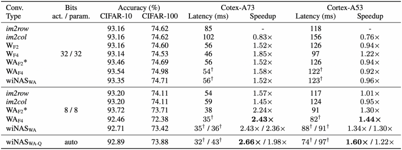Table 4: Accuracy on CIFAR-10 and CIFAR-100 and latency for A73 and A53 with a ResNet-18 architecture for various convolution algorithms and quantisation levels. Descriptions of convolutions: 
im2row / im2col — direct convolution 
$$\text{W}_\text{F2}$$ / $$\text{W}_\text{F4}$$ — Winograd convolution (not Winograd-aware) 
$$\text{WA}_\text{F2*}$$ — F2 for Winograd-aware with static transforms (F2-flex has no significant gain over F2) 
$$\text{WA}_\text{F4}$$ — F4 for Winograd-aware with learned transforms 
$$\text{wiNAS}_\text{WA}$$ / $$\text{wiNAS}_\text{WA-Q}$$ — wiNAS configurations (as described in previous section) 

There's a lot to unpack here, so let's break this table down bit by bit. First, we'll focus only on the latency values of A73; ignore A53 for now. The speedups are always measured w.r.t. to im2row in 32-bit. Let's start with the 32-bit experiments:

• Accuracy is barely impacted by Winograd convolutions. If anything, it even improves for Winograd-aware runs.
  
  
• F4 is faster than F2 as expected, but $$\text{WA}_\text{F4}$$ is somehow slower than $$\text{W}_\text{F4}$$. The reason for this is because the learned Winograd transforms are dense as opposed to static transforms, which are often relatively sparse. An in-depth discussion on this topic will be held in the next section.

Now, let's shift our attention towards the 8-bit experiments:

• Only by shifting from 32-bit to 8-bit, the speedup is 57%, roughly equivalent of replacing direct convolutions with Winograd convolutions.
  
  
• With only a slight hit on the accuracy (< 1% in CIFAR-10, < 2.5% on CIFAR-100), the speedup is 2.43x for $$\text{WA}_\text{F4}$$.
  
  
• Thus, we've demonstrated that with Winograd-aware layers, we can compound the speedups associated with Winograd and model quantisation, with minimal impact on the accuracy, on actual hardware.

Let's also quickly discuss the wiNAS runs (some of which have two latency values; left is for CIFAR-10, right for CIFAR-100):

• In 8-bit, $$\text{wiNAS}_\text{WA}$$ can recover some of the accuracy lost in $$\text{WA}_\text{F4}$$ with no impact on latency.
  
  
• The $$\text{wiNAS}_\text{WA-Q}$$ can further improve performance (as seen on CIFAR-10) and find different accuracy-latency trade-offs, although this is unfortunately not demonstrated here.
  
  
• wiNAS is not helpful in 32-bit.

Now, let's look at the experiments with the A53 CPU core.

• The speedups are much more modest here, especially in 32-bit. In this bit width, the Winograd-aware runs seem to hurt rather than help, especially when transforms are dense. The authors argue that this is due to the limited memory subsystem, preventing the A53 from efficient caching of large tensors.
  
  
• However, although we don't disagree with the above, we think the authors also missed an important observation: we see no speedup in im2row when using 8-bit instead of 32-bit, despite the arithmetic intensity having gone up. Recalling the roofline diagram, this implies that the inference task is compute-bound on the A53 (which, after all, is an efficiency core and not a performance core).
  
  
• In 8-bit, Winograd-aware layers generally give lower latencies, just like with A73. This indicates that the Winograd-aware layers can offer speedups across multiple platforms for lower-bit networks.

However, although we've seen benefits with Winograd-aware layers and wiNAS, we cannot stress enough that the biggest difference in latency/accuracy comes from hardware. If you compare the latency values across A73 and A53, we can measure speedups up to 2.5x. Therefore, we must take into account what hardware our application will be used on when implementing performance versus latency tests. This point may be trivial, but it's also extremely important.

Benchmarking CPU cores to characterise latency behaviour

As described in the section for wiNAS, the authors also benchmarked the two CPU cores on various input resolutions and channel sizes across the different convolution algorithms, in order to characterise the latency behaviour. The result table is not included in this blog because it's fairly cluttered (refer to Figure 8 in the paper instead), and frankly most takeaways were fairly trivial (latency increasing with larger input dimensions and channel sizes, etc.). However, there were a couple of interesting observations, both of which is evident from Figure 10:

• Input layers do not seem to benefit from Winograd, since the number of input channels are too low to justify using Winograd instead of direct convolution;
  
  
• Winograd input and output transforms are costly and may consist of over 25% of the overall latency. The behaviour here seems to be very hardware dependent, and may relate to the available memory bandwidth on each system.

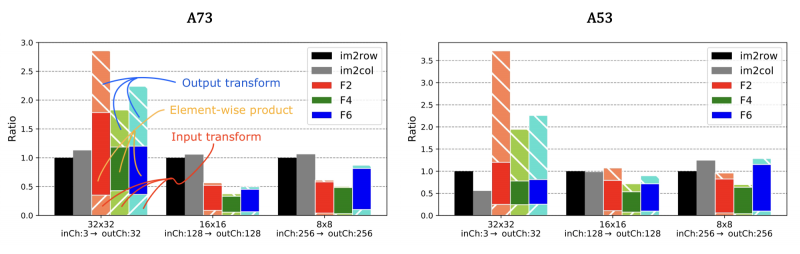Figure 10: Latencies to execute different layers in a 32-bit ResNet-18 network with static Winograd transforms. Left: A73. Right: A53. 
The solid colour bar regions represent the element-wise multiplication stage of the Winograds, whereas the portion below it represents the input transform and the portion above it the output transform. 

Discussion 

Dense Winograd transforms

The default static Winograd transforms $$\mathbf{B}^T$$, $$\mathbf{G}$$ and $$\mathbf{A}^T$$ are relatively sparse. Example for F4 can be seen below. Multiple implementations of matrix-matrix multiplications, such as Arm's Compute Library, can exploit data sparsity which often results in lower latencies.

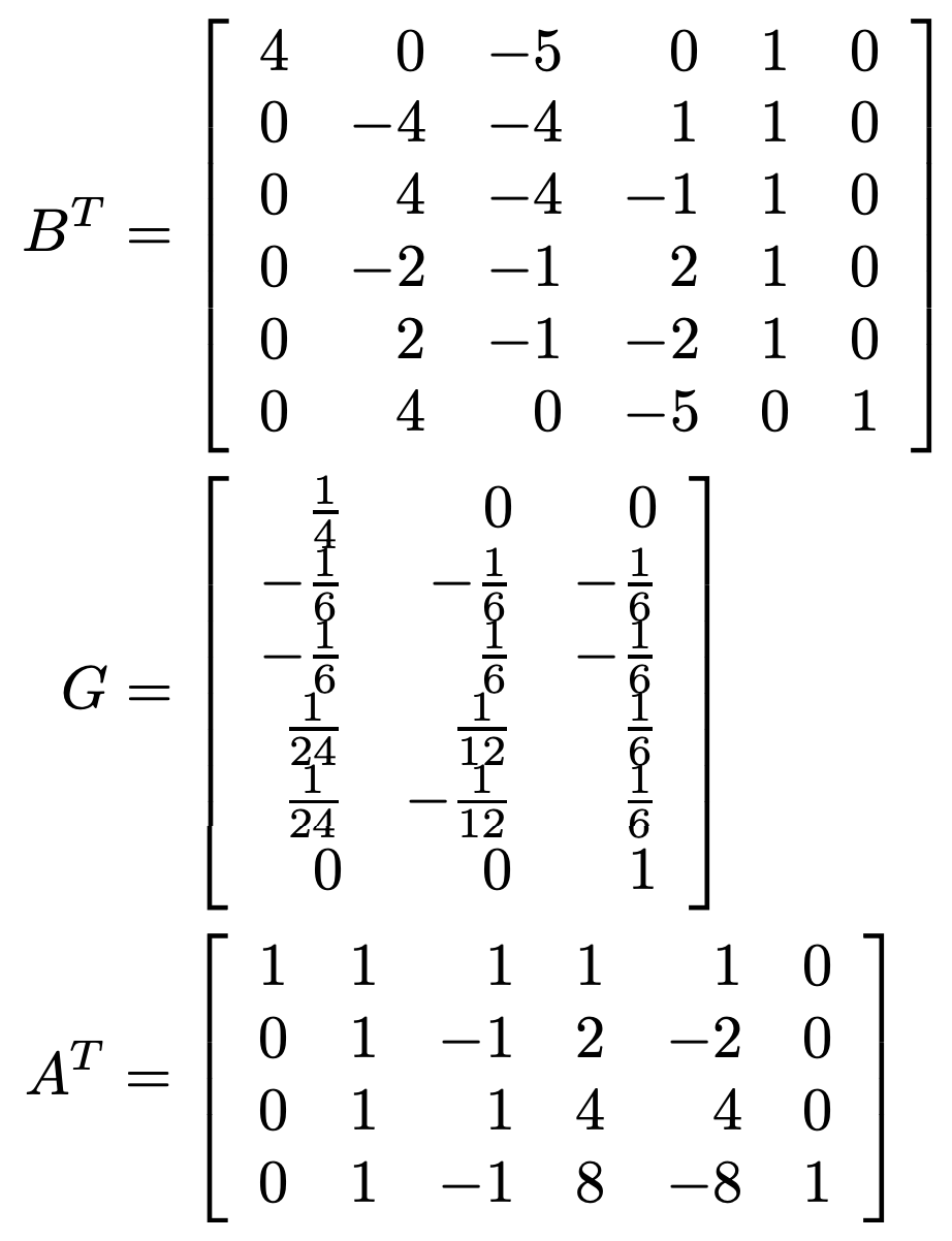Figure 11: Default Winograd transformation matrices for F4, as initialised by the Cook-Toom algorithm. [4]

When Winograd-aware layers learn flexible transforms, it is very unlikely that the resulting matrices are sparse. However, due to the runtime being mostly determined by data movement, the incurred penalty is less severe for memory-bound applications, where additional computation can be tolerated without necessarily increasing execution time.

Moving forwards

The images used in this study are relatively small; it is uncertain how much of this knowledge is transferable to problem domains involving high-resolution images, especially for the actual hardware tests. Another interesting aspect is whether the speedups involved also apply to GPUs and NPUs, which have very different execution structures to CPUs.

Whilst the wiNAS framework seems exciting, we are uncertain of how successful these experiments actually were. The authors claim that the framework can be used to jointly optimise for accuracy and latency, but they show no such trade-off curve which would have been very interesting to look at.

Lastly, there still seems to be issues associated with F6, since it is omitted from the resulting wiNAS architectures as well as the final accuracy vs runtime table. We suspect that there is still accuracy issues with F6 in low-bit models, which Winograd-aware training cannot remedy well enough; we would need further innovation in this space to enable the usage of F6 Winograds.

References

[1] Sze, V., Chen, Y. H., Yang, T. J. & Emer, J. (2017) Efficient Processing of Deep Neural Networks: A Tutorial and Survey. https://arxiv.org/pdf/1703.09039.pdf

[2] Zlateski, A., Jia, Z., Li, K. & Durand, F. (2018) FFT Convolutions are Faster than Winograd on Modern CPUs, Here is Why. https://arxiv.org/pdf/1809.07851.pdf

[3] Maji, P., Mundy, A., Dasika, G., Beu, J., Mattina, M. & Mullins, R. (2019) Efficient Winograd or Cook-Toom Convolution Kernel Implementation on Widely Used Mobile CPUs. https://arxiv.org/pdf/1903.01521.pdf

[4] Toom, A. L. (1963) The complexity of a scheme of functional elements realizing the multiplication of integers. http://toomandre.com/my-articles/engmat/MULT-E.PDF

[5] Cai, H., Zhu, L. & Cai, S. H. (2019) ProxylessNAS: Direct Neural Architecture Search on Target Task and Hardware. https://arxiv.org/pdf/1812.00332.pdf

[6] He, K., Zhang, X., Ren, S. & Sun, J. (2015) Deep Residual Learning for Image Recognition. https://arxiv.org/pdf/1512.03385.pdf

[7] LeCun, Y., Bottou, L., Bengio, Y. & Haffner, P. (1998) Gradient-Based Learning Applied to Document Recognition. http://yann.lecun.com/exdb/publis/pdf/lecun-98.pdf

[8] Chen, T., Xu, B., Zhang, C. & Guestrin, C. (2016) Training Deep Nets with Sublinear Memory Cost. https://arxiv.org/pdf/1604.06174v2.pdf

[9] Barabasz, B., Anderson, A., Soodhalter, K. M. & Gregg, D. (2018) Error Analysis and Improving the Accuracy of Winograd Convolution for Deep Neural Networks. https://arxiv.org/pdf/1803.10986.pdf