In this blog, Chri Besenbruch and Vira Koshkina look at Bits-back coding - a lossless data compression method, first introduced in 1997, in the paper "Efficient Stochastic Source Coding and an Application to a Bayesian Network Source Model". We review the fundamental principles and look at state-of-the-art implementations. 

1. Introduction

The amount of data on the internet increases yearly, thus increasing the bandwidth required for transferring it. Fundamentally, compression is a process that encodes the original data into a representation that takes fewer bits than the original data. With more data coming from different sources, effective compression methods are needed. Compression algorithms can be broadly split into lossless compression and lossy compression. In the lossless case, the filesize of the original data is reduced during data compression (encoding), but the data can be restored exactly after decompression (decoding). On the other hand, in lossy compression, some data, usually unnoticeable to the user, is lost in the encoding process. 

In general terms, the compression process can be split into two stages: the sender first encodes the data $$x$$ that they want to send into a bitstream with the smallest possible number of bits, then the receiver gets the bitstream and decodes it to reconstruct $$x$$. In the case of lossless compression, the $$x$$ must be reconstructed precisely.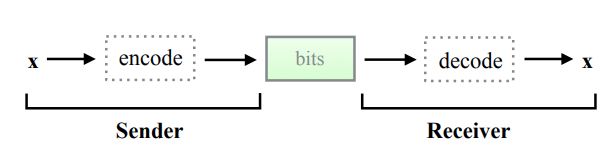Figure 1: Overview of lossless compression. First, the sender encodes data $$x$$ to a code with the smallest possible number of bits with no information loss. The receiver decodes this code and reconstructs $$x$$ exactly. From [3] Figure 1.

Most existing lossy compression algorithms operate by first transforming the data $$x$$ into a suitable continuous-valued representation $$y$$, quantising its elements and then encoding the discrete representation of $$y$$ losslessly into the bitstream. On the other side, the receiver starts by reconstructing the discretised version of  $$y$$ exactly and then uses it to restore the initial data $$x$$ approximately.  

Entropy coding relies on a prior probability model of the quantised representation, known to both the encoder and decoder (the entropy model). 

This blog post will look at a form of lossless data compression: "Neural Bits-Back coding". This blog's purpose is to give an introduction and an overview of the topic and high-level explanations of papers that introduce and develop this concept [1-5] and also look at the implementation and performance of state-of-the-art methods [6-12].

1.1. Notations 

Let us begin by clarifying the notation that we will be using in this post and how their equivalents in the papers served as the basis for it.

We shall briefly detail some fundamental concepts of Information Theory and compression before proceeding with Bits-Back coding.

2. Entropy and compression

The smallest possible bitrate of losslessly compressed data $$y$$, with some distribution $$p_y$$ is entropy:

 $$H(y) = -E_{p(y)}[\log\;p(y)].$$

In the general case, computing $$p(y)$$ is impossible, and achieving the optimal bitrate $$H(y)$$ is not feasible. To overcome this, we have to resort to approximating $$p(y)$$ using some other distribution, which increases the size of the final bitstream causing an approximation gap.

2.1 Latent variable models

A latent variable model is one of the methods used when we do not have direct access to $$p(y)$$. In this case, we condition $$y$$ on some latent variable $$z$$ while ensuring that the conditional distribution $$p(y\;|\;z)$$ is tractable. For example, consider linear regression as the simplest case of a latent variable model.  While the marginal distribution of explaining variable $$p(y)$$ is unknown, with observed data $$y$$ and latent variables $$z$$. In the traditional formulation, $$y = β z + ϵ $$ where $$ϵ $$ is a residual which is assumed to be normally distributed. 

In the case of compression, $$z$$ is an unobserved latent variable, which is usually obtained using a HyperPrior model in AI-based lossy compression [2].  The downside is that now we pass $$z$$ we used for conditioning to the receiver, meaning that we have to encode it into bitstream with the prior distribution $$p(z)$$.

So, how does it work? 

Suppose we have access to $$p(y\;|\;z)$$ and $$p(z)$$. Here, we construct a latent variable model $$p(y,z)$$ which is typically executed as $$p(y\;|\;z) \cdot p(z)$$. In short, we compress the latent variable $$z$$ given some prior $$p(z)$$ distribution and afterwards compress $$y$$ given $$z$$ using $$p(y\;|\;z)$$. The decoding side executes the same process in reverse. Using latent variable models, our entropy model for $$p(y)$$ becomes a joint entropy model of $$p(y,z)$$. 

The entropy of $$p(y,z) = p(y\;|\;z)p(z)$$ is then equal to:

 $$H(y,z) = -E_{p(y,z)}[\log p(y,z) ]= -E_{p(y,z)}[ \log p(y\;|\;z) + \log p(z)]$$

$$= -E_{p(y\;|\;z)} [ \log p(y\;|\;z) ] - E_{p(z)}[ \log p(z)]= \color{green} H(p(y\;|\;z)) \color{blue} +H(p(z))$$

The first term in this summation (coloured green) is the size of the bitstream for encoding $$y$$ using the distribution $$p(y\;|\;z)$$ and the second term (coloured blue) is the size of the bitstream for $$z$$ encoded with distribution $$p(z)$$.

2.2. Why is it not optimal?

It makes sense that in most cases $$H(p(y,z)) > H(p(y))$$as there is more information that needs to be encoded. We can quantify how large this difference is. For that let's look at the conditional distribution $$p(y\;|\;z)$$. Using Bayes rule, we can represent it as:

$$p(y\;|\;z) = \frac{p(z\;|\;y)p(y)}{p(z)}$$

We then can rewrite $$p(y)$$ as:

$$p(y) = \frac{p(y\;|\;z)p(z)}{p(z\;|\;y)}$$

The entropy of $$y$$ under this formulation is then: 

 $$H(y) = -E_{p(y)}\left[\log \frac{p(y\;|\;z)p(z)}{p(z\;|\;y)}\right]$$

$$= -E_{p(y,z)}[\log p(y\;|\;z) +\log p(z) - \log p(z\;|\;y)]$$

$$= -E_{p(y,z)} [ \log p(y\;|\;z) ]   - E_{p(y,z)}[\log p(z)] + E_{p(y,z)}[\log p(z\;|\;y)]$$

$$= \color{green} H(p(y\;|\;z))  \color{blue} + H(p(z)) \color{red}- H(p(z\;|\;y))$$

The first two terms, coloured green and blue, correspond to the terms in the equation above, but the third term, coloured in red, is negative, which means that having it in the equation reduces the size of the bitstream. This term is where the gains from using bits-back coding, formulated in terms of the conditional probability $$p(y\;|\;z)$$, are coming from.

In short, by using a latent variable model, we overestimate the length of the message by $$H(p(z\;|\;y))$$ bits. Bits-back coding addresses this overestimation by using a form of latent variable encoding that estimates $$p(y)$$ instead of $$p(y, z)$$.

3. What is in the bitstream?

Consider the components of the bitstream after encoding discrete data $$y$$; see Figure 2. Each of the components represents additional bits required to encode the data:

1. Entropy H(y) - the minimal bitrate the data $$y$$ can take if we had access to the true distribution $$p(y)$$.

2. Approximation gap - introduced by the fact that marginal distribution $$p(y)$$ is not known and has to be approximated.

3. KL gap - $$D_{KL}(q(z\; |\; y)\;||\; p(z \;| \;y))$$ - introduced by using the approximation $$q(z \;|\; y)$$ to the true posterior $$p(z\; |\; y)$$.

4. Dirty bits - introduced by the fact that the number of bits must be an integer. For example, even if the theoretical shortest length is 11.2 bits, the bitstream will be 12 bits - the shortest realisable length. The difference, 0.8, is the length of the dirty bits. Dirty bits typically take less than 1% of the total bitstream size.

5. Initial bits - initial bits that are required for bits-back coding. These will be addressed later.

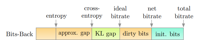Figure 2: Components of a bitstream with Bits-back coding. From [5] Figure 1.  

Bits-back coding is all about removing the approximation Gap (minimising the ELBO), including consideration of the initial bits. Bits-back coding does not relate to the KL-Gap or the dirty bits.

3.1. Advanced concepts - KL-gap

In general, computing the true posterior distribution $$p(z\;|\;y)$$ is not feasible. Therefore, we have to approximate it with $$q(z\;|\;y)$$. Then, the minimum message length becomes: 

$$E_{q(z\;|\;y)}[ \; - \log p(y\;|\;z) - \log p(z) + \log q(z\;|\;y)]$$

$$ = E_{q(z\;|\;y)}[  \;-\log p(y,z) + \log q(z\;|\;y)]$$

$$=  E_{q(z\;|\;y)}[\;  -\log (p(z\;|\;y)p(y))  + \log q(z\;|\;y)]$$

$$= E_{q(z\;|\;y)}[\;  - \log p(z\;|\;y) - \log p(y) + \log q(z\;|\;y)]$$

$$=  E_{q(z\;|\;y)}\left[  -\log p(y) + \log \frac{q(z\;|\;y)}{p(z\;|\;y)}\right]$$ 

$$= E_{q(z\;|\;y)}[ \; - \log p(y)] + D_{KL}(q(z\;|\;y) \;||\;  p(z\;|\;y))$$

Moving $$\log p(y)$$ to the left we get: 

$$\log p(y) = -\;E_{q(z\;|\;y)}\left[ \log\frac{p(y,z)}{q(z\;|\;y)}\right] + E_{q(z\;|\;y)}\left[\log\frac {q(y,z)}{p(z\;|\;y)}\right]$$

$$=ELBO$$ + $$D_{KL}(q(z\;|\;y) \;||\;  p(z\;|\;y))$$ 

The discrepancy between distributions $$p(z\;|\;y)$$ and $$q(z\;|\;y)$$ adds approximately $$D_{KL}(q(z \;| \;y) \;||\; p(z \;| \;y))$$ bits to the final bitrate and is called KL-gap.

Since the second term, KL-gap is non-negative $$D_{KL}(q(z\;|\;y) \;||\;  p(z\;|\;y))>=0$$, the first term,  $$E_{q(z\;|\;y)} \left[ \log\frac{p(y,z)}{q(z\;|\;y)} \right]$$ is the Evidence Lower Bound (ELBO), a lower bound on $$\log p(y)$$. ELBO is the approximation gap in Figure 3.  

Bits-back coding is only concerned with minimising the ELBO part of this equation, which reduces the approximation gap without addressing the KL-gap.  Therefore, for simplicity, we will assume that the Bits-back coding has access to $$p(z\;|\;y)$$ in the remainder of this blogpost.

4. Bits back coding - Introduction

Bits-back coding is a form of lossless compression that addresses the entropy overestimation of using latent variable models. Bits-back coding uses a form of latent variable encoding that tightly estimates $$p(y)$$ instead of the joint distribution $$p(y,z)$$.

For a recap of latent variable models, see sections 2.1 and 2.2. 

In Bits-back coding, we want to model $$p(y)$$, which is infeasible. Suppose we have access to $$p(y\;|\;z)$$, $$p(z)$$ and $$p(z\;|\;y)$$. Then, Bits-back coding lets us formulate a latent variable model that evaluates to $$H(p(y))$$. On a high level, the idea is to use $$p(y\;|\;z)$$ and $$p(z)$$, the same as in latent variable models, but also utilise $$p(z\;|\;y)$$, not the same as in latent variable models. We can write $$H(p(y))$$ as $$H(p(y\;|\;z)) + H(p(z)) - H(p(z\;|\;y))$$. Thus, using all three distributions, we can go from $$H(p(y,z))$$ to $$H(p(y))$$ and close the overestimation gap of $$H(p(z\;|\;y))$$. 

Before going into more detail, let's first build an intuition about how these terms relate to the bitstream:

• $$+H(p(y\;|\;z))$$ and $$+H(p(z))$$ are positive. If the Encoder sees these terms, they push data onto the bitstream, making it longer and increasing filesize. If the Decoder sees these terms, they pop data from the bitstream, making the remaining bitstream shorter and recovering data.
  
  
• $$-H(p(z\;|\;y))$$ is negative. If the Encoder sees these terms, they pop data from the bitstream, making the remaining bitstream shorter and recovering data. If the Decoder sees these terms, they push data onto the bitstream, making it longer and increasing filesize.

Therefore, during encoding, we no longer simply build a bitstream by pushing data onto it. In fact, during encoding, we pop $$-H(p(z\;|\;y))$$ and push data $$+H(p(y\;|\;z))$$ and $$+H(p(z))$$. The same holds for decoding. This might look not very clear initially, but it's an integral part of Bits-back coding. The Encoder and Decoder both push and pop data from the bitstream.

5. Bits-back coding - Encoding, Decoding (Inference)

Figure 3 illustrates an encoding/decoding step.

1. There is some initial bitstream. We'll talk about this more later, but for now, note that if we want to compress $$img$$ this initial bitstream can be unrelated to it. It could just be noise.

2. The Sender wants to send $$y$$. The Sender has $$y$$, $$z$$, $$p(y\;|\;z)$$, $$p(z)$$ and $$p(z\;|\;y)$$.

3. The Sender uses the initial bitstream and decodes a variable $$z$$ using $$p(z\;|\;y)$$. The Sender pops data of the bitstream.

4. The Sender encodes $$y$$ using $$p(y\;|\;z)$$ and pushes this information onto the bitstream.

5. The Sender encodes $$z$$ using $$p(z)$$ and pushes this information onto the bitstream.

After the bitstream is sent:

1. The Receiver has access to $$p(y\;|\;z)$$, $$p(z)$$ and $$p(z\;|\;y)$$.

2. The Receiver gets the bitstream and decodes $$z$$ using $$p(z)$$. The Receiver pops data off the bitstream.

3. The Receiver decodes $$y$$ using $$p(y\;|\;z)$$. The Receiver pops data off the bitstream.

4. The Receiver encodes $$z$$ using $$p(z\;|\;y)$$. The Receiver pushes data onto the bitstream.

5. The receiver has successfully decoded the $$img$$ and has recovered the initial bitstream, which the Sender used in step 1.

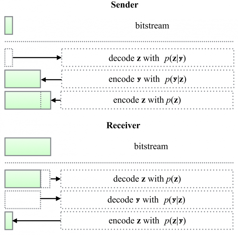Figure 3: Encoding and Decoding using Bits-Back Coding. Modified from [3] Figure 3.

Note, there is a fundamental concept happening at the Sender step 3. We are decoding some unrelated, initial bitstream using $$p(z\;|\;y)$$ to get $$z$$. What does this do? 

If we encode some data $$x$$ into a bitstream using $$p(x)$$ and then decode the bitstream using the same distribution $$p(x)$$, we get back $$x$$. Encoding and decoding using the same distribution, reverse push/pop order.

If we encode some data $$x$$ into a bitstream using $$p(x)$$ and then decode the bitstream using a different distribution $$p(y\;|\;z)$$, it is equivalent to sampling from $$p(y\;|\;z)$$. Encoding and decoding using different distributions, reverse push/pop order.

Thus, the Sender step 3 is equivalent to sample a $$z$$ from $$p(z\;|\;y)$$, but the sampling is not random but deterministically fixed by the initial bitstream. You can think of it as the initial bitstream fixing a seed.

Quoting the authors of [3]:

To understand this, we have to clarify what "decoding" means. If the model fits the true distributions perfectly, entropy coding can be understood as a (bijective) mapping between datapoints and uniformly random distributed bits. Therefore, assuming that the bits are uniformly random distributed, decoding information z from the bitstream can be interpreted as sampling z.

The above example shows encoding and decoding for a Bits-back coding algorithm with a latent variable model with a depth of 1, similar to a HyperPrior model. However, Bits-back coding works with arbitrary hierarchical dimensions. For instance, it is naively extendable to a HyperHyperPrior or a HyperHyperHyperPrior model. Figure 4 illustrates a hierarchical model of depth 3, with hidden latent variable $$z_1$$, $$z_2$$ and $$z_3$$.

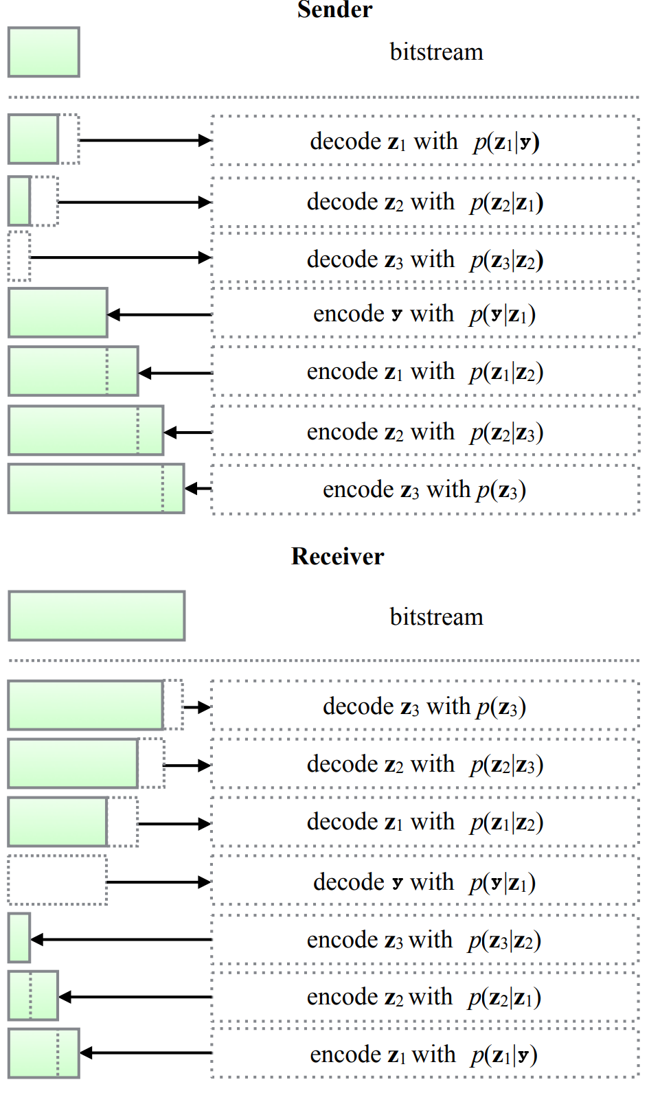Figure 4: Illustrating Bits-Back Coding with higher hierarchical modelling. Modified from [3] Figure 5.

6. Bits-back coding - Naive Example (Training)

After we've discussed encoding and decoding, aka. inference, how do we train an AI-based Bits-back coding pipeline? Let's recall the essential assumptions:

1. We are talking about lossless compression. Let's say lossless image compression.

2. We assume we have access to $$p(y\;|\;z)$$, $$p(z)$$ and $$p(z\;|\;y)$$. 

3. If we decode an arbitrarily given bitstream using $$p(z\;|\;y)$$, it is the same as sampling a $$z$$ from the distribution.

A model that fulfils all of these properties is a double Variational AutoEncoder (see Figure 5). Suppose we have $$y$$ and an Encoder (neural network), which predicts $$μ_z$$ and $$σ_z$$. Then we sample a $$z$$ given $$N(μ_z, σ_z)$$ and pass $$z$$ through a Decoder (neural network), which predicts $$μ_y$$ and $$σ_y$$.

We have:  $$y  \;\text{~} \;p(y\;|\;z) = N(μ_y, σ_y) = N (Decoder(z))$$.

We have:  $$z \; \text{~} \;  p(z\;|\;y) = N(μ_z, σ_z) = N(Encoder(y))$$.

And we have some prior distribution over $$z\;  \text{~}\;  p(z) = N(0,1)$$.

The training steps are:

1. Get an image $$y$$ in discrete format (e.g. 0-255)

2. Pass $$y$$ through the Encoder to get $$μ_z, σ_z$$

3. Sample a $$z$$ from $$N(μ_z, σ_z)$$

4. Pass $$z$$ through the Decoder to get $$μ_y, σ_y$$

5. Calculate the Cross-Entropy $$H(p(y\;|\;z)) = H(N(y\;|\; μ_y, σ_y))$$

6. Calculate the Cross-Entropy $$H(p(z\;|\;y)) = H(N(z\;|\;μ_z, σ_z))$$

7. Calculate the Cross-Entropy $$H(p(z)) = H(N(z\;|\;0,1))$$

8. Total Loss: $$H(p(y\;|\;z)) + H(p(z)) - H(p(z\;|\;y))$$

9. Backwards pass through the neural networks, then repeat

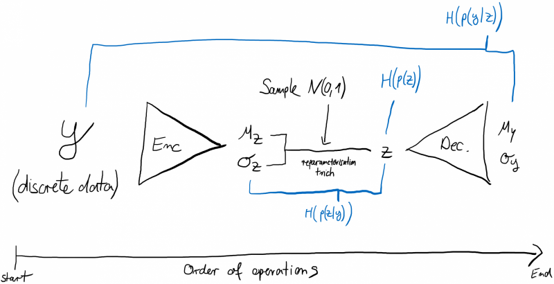Figure 5: Double AutoEncoder + Visualisation of the Losses used for Bits-Back Coding

Note how we have not made a quantisation assumption on $$z$$. Theoretically, Bits-back coding works with discrete $$y$$ and continuous $$z$$. However, in practice, there usually is a quantisation function applied to (the sampled) $$z$$, and it doesn't seem to make any difference.

Quoting the authors from [8]: 

Bits-back coding also works with continuous z discretized to high precision with negligible change in codelength. In this case, q(z|x) and p(z) are probability density functions. Discretizing z to bins z_hat of small volume delta_z and defining the probability mass functions Q(z_hat|x) and P(z_hat) by the method in Section 3.1, we see that the bits-back codelength remains approximately unchanged,

7. Bits-back coding - State-of-the-Art Implementations

briefly discuss how the two state-of-the-art papers, HiLLoC [6] and LBB [7], train their Bits-back coding pipeline. Both state-of-the-art approaches use the same Bits-back coding concept as described above. Note that the differences/improvements from these two methods come from their neural architecture and how it interacts with Bits-back coding.

HiLLoC uses a ResNet VAE architecture (RVAE). Note, "RVAE" is not a unique abbreviation in the ML community, it can have different meanings. An RVAE [11] combines a Resnet and Inverse Autoregressive Flow (IAF), chaining many small IAF networks together to build a hierarchical flow-based model for more flexible variational inference. Usecases are generative modelling (sampling from latent space distributions), compression (sending latent spaces), and density estimation.  The hierarchical nature of the RVAE is ideally suited for hierarchical Bits-back coding, as seen in Figure 4. With an RVAE, you get $$p(z\;|\;y)$$ via a forward pass, $$p(y\;|\;z)$$ via an inverse pass (IAF/flows are invertible) and $$p(z)$$ through a fixed prior; here being $$N(0,1)$$. Their code is available:  https://github.com/hilloc-submission/hilloc/tree/master/experiments

LBB uses a very similar setup to HiLLoC, but instead of an RVAE that chains together IAFs, they utilise the Flow++ network [12], a RealNVP-type flow with a dequantisation step. Their choice of normalising flow model is significantly more powerful as an RVAE but requires the calculation of the Jacobian at each hierarchical step. This results in better compression performance but significantly higher runtime. Their code is available: https://github.com/hojonathanho/localbitsback

8. Limitations

In Bits-back coding, we start encoding with a decoding step, requiring initial bits. During decoding, we get these initial bits back; and thus, the algorithm is called Bits-back coding. The initial bits are crucial as they guarantee the same sampling seed during encoding and decoding. There are three minor issues with the initial bits, which are often listed in literature: 

1. The initial bitstream's size needs to be sufficiently large to execute the full first decoding step at encoding, costing $$H(p(z\;|\;y))$$ bits. In hierarchical methods, the step costs $$H(p(z_1\;|\;y)) + H(p(z_2\;|\;z_1)) + ... + H(p(z_n\;|\;z_{n-1}))$$ bits. Some papers solve this by first encoding an image with FLIF, then Bits-back coding, or chopping the first image into blocks and encoding the first block with FLIF, the rest with Bits-back coding.
   
   

2. As the original bits act as a seed that guarantees the same sampling during encoding and decoding, a corruption to these bits breaks the entire Bits-back coding chain. We know that bit-flips or package corruption happens quite often when sending data. Therefore, chaining images/video frames together via having one act as initial bits for the next is very dangerous. There is no academic study that has looked into this issue yet.
   
   

3. The assumption of the initial bits is that they come from a perfect "encoding". This is equivalent to them being Bernoulli distributions with $$p=0.50$$. If this assumption does not hold, which it doesn't in practice, it adversely affects the encoding rate. Quoting the authors from [4]:

In our description of bits back coding in Section 2, we noted that the ‘extra information’ needed to seed bits back should take the form of ‘random bits’. More precisely, we need the result of mapping these bits through our decoder to produce a true sample from the distribution p(z | y). A sufficient condition for this is that the bits are i.i.d. Bernoulli distributed with probability 0.50 of being in each of the states 0 and 1. We refer to such bits as ‘clean’.

During chaining, we effectively use each compressed data point as the seed for the next. Specifically, we use the bits at the top of the ANS stack, which are the result of coding the previous latent according to the prior p(z). Will these bits be clean? The latent z is originally generated as a sample from q(z | y). This distribution is clearly not equal to the prior, except in degenerate cases, so naively we wouldn’t expect encoding  according to the prior to produce clean bits.

Some thoughts: While the limitation of the initial bit might sound challenging to overcome, there might be an easy fix: we could just communicate a sample seed for a pseudo-random generator at the start of our bitstream. Instead of using initial bits at encoding and decoding, the Sender/Receiver uses "the seed" to sample a $$p=0.50$$ Bernoulli distributed bitstream of arbitrary length, using it for popping $$p(z\;|\;y)$$.

Another practical limitation of Bits-back coding lies in its horrible runtime (see section 9 for numbers). Most papers cite compression performance for 64x64 crops, or more rarely 128x128 crops, at most. However, as far as I can tell, the horrible runtime is not necessarily an issue with the theoretical concept of Bits-back coding. Instead, it comes from the complex and autoregressive neural architectures the authors of [3], [4], [5], [6] and [8] use for distribution modelling. But it is striking that there are no neural Bits-back coding papers with fast and straightforward neural architectures; hinting that the concept relies on deep autoregressive models.

9. Bits-back coding - Performance

It is finally time to evaluate the performance of Bits-back coding algorithms. However, first a warning: The field is still very young with not too many papers published and a strongly yearly growth trajectory. Thus, current state-of-the-art results might underestimate the true potential of neural Bits-back coding.

The authors in [6] have a great result table:

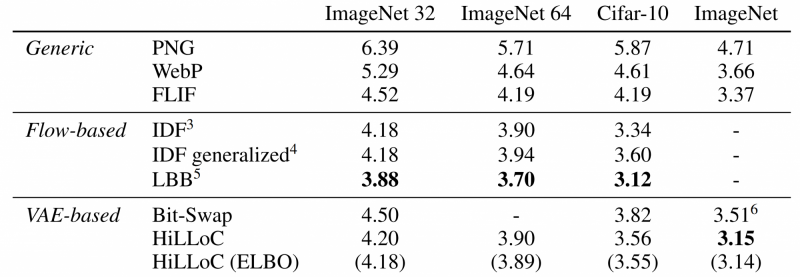Figure 6: Bits-Back Coding's Compression Performance

The table measures bits/dimensions with raw data having 8 bits per dimension (colour-image uint8). The table shows the best traditional lossless compression approach, namely PNG (1996), WebP (2010) and FLIF (2015). The table compares these approaches against the state-of-the-art Flow-based methods and the state-of-the-art RVAE-based Bits-back coding approaches. Note that the horrendous compression performance is due to compressing very low-resolution datasets. 

For the Flow-based methods, it's not a surprise to see the IDF paper [7], Integer Discrete Flow. The other approach, LBB [8] is the current state-of-the-art Bits-back coding approach (but very, very, very far away from real-time runtime). LBB combines Flow-based methods with Bits-back coding.

For the RVAE-based method, the table shows Bit-Swap [3], one of the first papers demonstrating the feasibility of neural Bits-back coding. And the table shows HiLLoC, a more runtime-oriented Bits-back coding approach (still, far away from real-time).

The results indicate that neural Bits-back coding can hold its own against traditional, lossless compression. In fact, LBB consistently reaches 15% to 25% lower filesize. For runtime, this looks very different. Getting reliable runtime results is very difficult, as the hardware platform and the quality of implementation massively impacts the outcome. The "faster" Bits-back coding algorithm "HiLLoC" reports runtimes of >1 seconds for 128x128 images on a desktop with 6 CPUs and a GTX 1060 GPU. The best-performing Bits-back coding algorithm "LBB" reports decoding times of 1351 seconds for a 64x64 image for its best variant (performance in Figure 6) and 0.71 seconds for a 64x64 image for a speedy version (resulting in compression performance hit). In short, Bits-back coding will not run in real-time any time soon.

10. Comparison to Other Approaches 

When trying to evaluate the performance of Bits-back coding approaches, the essential question is how it performs against traditional methods (answered in Figure 6) and how it performs against other neural network approaches. This section covers the latter.

Unfortunately, it is tough to find fair comparisons in literature. Bits-back coding methods typically evaluate using low-resolution datasets (e.g. ImageNet 32x32 or 64x64), whereas more VAE-based methods tend to benchmark using the Kodak dataset.

The paper [9] reports a more Balle oriented VAE-based approach to lossless compression and reports the following results: 

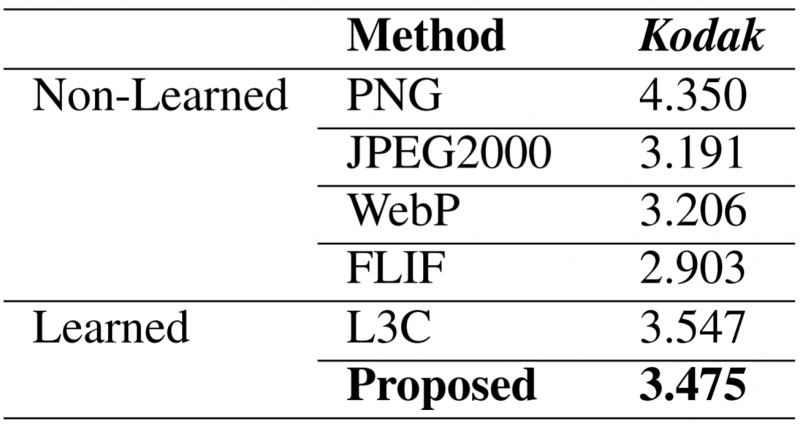Figure 7: Lossless Compression Results from [9]

The results on Kodak from [9] are 108% as large as WebP (so worse than WebP). The Bits-back coding approach HiLLoC is 84% (3.90/4.64) as large as WebP on ImageNet64 and 86% (3.15/3.66) as large as WebP on ImageNet. The Bits-back coding approach LBB is 80% (3.70/4.64) as large as WebP on ImageNet64.

The paper [10] uses a more Balle oriented VAE-based approach in combination with Wavelets and reports the following results: 

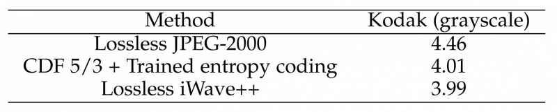Figure 8: Lossless Compression Results from [10]

Note that Lossless JPEG-2000 is evenly matched with WebP. Thus, Lossless iWave++ results are roughly 89% (3.99/4.46) as large as WebP on Kodak Grayscale.

Ultimately, we have around 85% filesize against WebP for "semi-fast" Bits-back coding methods and 80% filesize against WebP for slow Bits-back coding methods. In contrast, we have 108% filesize against WebP for "superfast" VAE-based methods and 89% filesize against WebP for "semi-slow" VAE-based methods. It looks as if Bits-back coding has a slight edge in lossless compression performance. Still, this edge comes with absurd runtime requirements, limiting the approach to very, very small resolutions.

11. Personal Thoughts

While Bits-back coding methods show impressive lossless compression gains, I wonder how much of the gains come from using Bits-back coding and how much is due to using powerful neural network models. For instance, LBB uses Flow++, a very strong neural network-based density modelling method.

I am also hesitant to accept the theoretical justification of using Bits-back coding, or at least I would question whether there is a need in practice for it. The main idea of Bits-back coding is that latent variable models don't approximate $$p(y) = p(y\;|\;z) \cdot p(z) \cdot p(z\;|\;y) ^{-1}$$ sufficiently well, because latent variable models approximate $$p(y,z) = p(y\;|\;z) \cdot p(z)$$; which is not the same. While this is valid, if we have a deterministic function that maps a $$y$$ latent to a $$z$$ latent, e.g. $$HyperEncoder(y) = z$$, then $$p(z\;|\;y) = 100\%$$. In such a scenario, $$p(y) == p(y,z)$$, and there are limited gains of using Bits-back coding over traditional latent variable modelling.

Therefore, in my opinion, Bits-back coding looks like a method that still tries to accomplish compression using naive VAEs (or Flows). However, the field has moved onwards, nowadays using VAE-related approaches to compression with a fixed $$z$$ latent; see Balle's work [2]. Therefore, I don't think Bits-back coding has a future (especially not, considering all its other limitations).

12. References

[1] Frey, Brendan J., and G. E. Hinton. "Efficient stochastic source coding and an application to a Bayesian network source model." Computer Journal (1997). http://www.cs.toronto.edu/~fritz/absps/freybitsback.pdf

[2] Ballé, J., Minnen, D., Singh, S., Hwang, S. J., & Johnston, N. "Variational image compression with a scale hyperprior". arXiv preprint arXiv:1802.01436 (2018). https://arxiv.org/pdf/1802.01436v2.pdf

[3] Kingma, Friso, Pieter Abbeel, and Jonathan Ho. "Bit-swap: Recursive bits-back coding for lossless compression with hierarchical latent variables." International Conference on Machine Learning. PMLR, (2019). https://arxiv.org/pdf/1905.06845.pdf

[4] Townsend, James, Tom Bird, and David Barber. "Practical lossless compression with latent variables using bits back coding." arXiv preprint arXiv:1901.04866 (2019). https://arxiv.org/pdf/1901.04866.pdf

[5] Ruan, Yangjun, et al. "Improving Lossless Compression Rates via Monte Carlo Bits-Back Coding." arXiv preprint arXiv:2102.11086 (2021). https://arxiv.org/pdf/2102.11086.pdf

[6] Townsend, James, et al. "Hilloc: Lossless image compression with hierarchical latent variable models." arXiv preprint arXiv:1912.09953 (2019). https://arxiv.org/pdf/1912.09953.pdf

[7] Hoogeboom, Emiel, et al. "Integer discrete flows and lossless compression." arXiv preprint arXiv:1905.07376 (2019). https://arxiv.org/abs/1905.07376

[8] Ho, Jonathan, Evan Lohn, and Pieter Abbeel. "Compression with flows via local bits-back coding." arXiv preprint arXiv:1905.08500 (2019). https://arxiv.org/abs/1905.08500 

[9] Cheng, Zhengxue, et al. "Learned Lossless Image Compression with A Hyperprior and Discretized Gaussian Mixture Likelihoods." ICASSP 2020-2020 IEEE International Conference on Acoustics, Speech and Signal Processing (ICASSP). IEEE, 2020. https://arxiv.org/pdf/2002.01657.pdf 

[10] Ma, Haichuan, et al. "End-to-End Optimized Versatile Image Compression With Wavelet-Like Transform." IEEE Transactions on Pattern Analysis and Machine Intelligence (2020). Paper: Upload_to_Blog_09204799.pdf 

[11] Kingma, Diederik P., et al. "Improved variational inference with inverse autoregressive flow. 2016." Google Scholar Google Scholar Digital Library Digital Library. https://arxiv.org/pdf/1606.04934.pdf

[12] Ho, Jonathan, et al. "Flow++: Improving flow-based generative models with variational dequantisation and architecture design." International Conference on Machine Learning. PMLR, 2019. https://arxiv.org/abs/1902.00275